Simultaneous Object Pose and Velocity Computation Using a Single View from a Rolling Shutter Camera Omar Ait-Aider, Nicolas Andreff, Jean Marc Lavest, and Philippe Martinet Universit´e Blaise Pascal Clermont Ferrand, LASMEA UMR 6602 CNRS
[email protected], WWW home page: http://www.lasmea.fr
Abstract. An original concept for computing instantaneous 3D pose and 3D velocity of fast moving objects using a single view is proposed, implemented and validated. It takes advantage of the image deformations induced by rolling shutter in CMOS image sensors. First of all, after analysing the rolling shutter phenomenon, we introduce an original model of the image formation when using such a camera, based on a general model of moving rigid sets of 3D points. Using 2D-3D point correspondences, we derive two complementary methods, compensating for the rolling shutter deformations to deliver an accurate 3D pose and exploiting them to also estimate the full 3D velocity. The first solution is a general one based on non-linear optimization and bundle adjustment, usable for any object, while the second one is a closed-form linear solution valid for planar objects. The resulting algorithms enable us to transform a CMOS low cost and low power camera into an innovative and powerful velocity sensor. Finally, experimental results with real data confirm the relevance and accuracy of the approach.
1
Introduction
In many fields such as robotics, automatic inspection, road traffic, or metrology, it is necessary to capture clear images of objects undergoing high velocity motion without any distortion, blur nor smear. To achieve this task, there is a need to image sensors which allow very short exposure time of all the matrix pixels simultaneously. This functionality requires a particular electronic design that is not included in all camera devices. Full Frame CCD sensors, without storage memory areas, require mechanical obturator or stroboscopic light source, introducing more complexity in the vision system. Frame Transfer CCD sensors may not reach the desired frame rate or may be costly because of additional sillicium in storage areas [9]. Standard CMOS Rolling Shutter sensors are considered as low cost and low power sensors. They are becoming more frequently used in cameras. They enable adequate exposure time without reducing frame rate thanks to overlapping exposure and readout. Their drawback is that they distort images of moving
objects because the pixels are not all exposed simultaneously but row by row with a time delay defined by the sensor technology (figure 1). This distortion may represent a major obstacle in tasks such as localization, reconstruction or default detection (the system may see an ellipse where in fact there is a circular hole). Therefore, CMOS Rolling Shutter cameras could offer a good compromise between cost and frame rate performances if the problem of deformations is taken into account.
Fig. 1. An example of distortion of a rotating ventilator observed with a Rolling Shutter camera: static object (right image) and moving object (left image).
2
Related works and contributions
This work, is related to our previous one presented in [1], which focused on the development of a method which maintains accuracy in pose recovery and structure from motion algorithms without sacrificing low cost and power characteristics of the sensor. This was achieved by integrating, in the perspective projection model, kinematic and technological parameters which are both causes of image deformations. The resulting algorithm, not only enables accurate pose recovery, but also provides the instantaneous angular and translational velocity of observed moving objects. Rolling shutter effects which are considered as drawbacks are transformed into an advantage ! This approach may be considered as an alternative to methods which uses image sequences to estimate the kinematic between views since it reduces the amount of data and the computational cost (one image is processed rather than several ones). In a parallel work by Meingast [7] (published after the submission of this paper), the projection in rolling shutter cameras is modelled in the case of fronto-parallel motion obtaining equations which are similar to those of Crossed-Slits cameras [13]. To our knowledge, there is no work in the vision community literature on taking into account effects of rolling shutter in pose recovery algorithms nor on computing velocity parameters using a single view. Indeed, all pose recovery methods ([6], [8], [2], [3], [10]) make the assumption that all image sensor pixels are exposed simultaneously. The work done by Wilburn et al. [11] concerned the correction of image deformation due to rolling shutter by constructing a single image using several images from a dense camera array. Using the knowledge of the time
delay due to rolling shutter and the chronograms of release of the cameras, one complete image is constructed by combining lines exposed at the same instant in each image from the different cameras. Two main contributions are presented in this paper. First, the perspective projection model of rolling shutter cameras presented in [1] is improved by removing the assumption of small motion during image acquisition. This makes the model more accurate for very fast moving objects. A novel non-linear algorithm for pose and velocity computation is then described. It generalizes the bundle adjustment method to the case of moving points. Indeed, it is based on non-linear least-square optimization of an error function defined in image metric and expressed with respect to both pose and velocity parameters (rather than to only pose parameters in classical approaches). Second, a linear algorithm for pose and instantaneous velocity computation is developed in the particular case of planar objects. This linear solution provides an initial estimate of the pose and velocity parameters and serves to initialize the non-linear algorithm. Section 3 of this paper describes the process of image acquisition using a CMOS Rolling Shutter imager. In section 4, a general geometric model for the perspective projection of 3D point on a solid moving object is presented. Image coordinates of the point projections are expressed with respect to object pose and velocity parameters and to the time delay due to image scanning. Section 5 deals with the problem of computing pose and velocity parameters of a moving object, imaged by a Rolling Shutter camera, using point correspondences. Finally, experiments with real data are presented and analyzed in section 6.
3
What is rolling shutter ?
In digital cameras, an image is captured by converting the light from an object into an electronic signal at the photosensitive area (photodiode) of a solid state CCD or CMOS image sensor. The amount of signal generated by the image sensor depends on the amount of light that falls on the imager, in terms of both intensity and duration. Therefore, an on-chip electronic shutter is required to control exposure. The pixels are allowed to accumulate charge during the integration time. With global shutter image sensors, the entire imager is reset before integration. The accumulated charge in each pixel is simultaneously transferred to storage area. Since all the pixels are reset at the same time and integrate over the same interval there is no motion artifacts in the resulting image. With a CMOS image sensor with rolling shutter, the rows of pixels in the image are reset in sequence starting at the top and proceeding row by row to the bottom. The readout process proceeds in exactly the same fashion and the same speed with a time delay after the reset (exposure time). The benefit of rolling shutter mode is that exposure and readout are overlapping, enabling full frame exposures without reducing the frame rate. Each line in the image has the same amount of integration, however the start and end time of integration is shifted in time as the image is scanned (rolled) out of the sensor array as shown in Fig.2.
In this case, if the object is moving during the integration time, some artifacts may appear. The faster the object moves the larger is the distortion.
Fig. 2. Reset and reading chronograms in rolling shutter sensor (SILICON IMAGING documentation).
4
Projecting a point with rolling shutter camera
Let us consider a classical camera with a pinhole projection model defined by its intrinsic parameter matrix [10] αu 0 u0 K = 0 αv v0 0 0 1 T
Let P = [X, Y, Z] be a 3D point defined in the object frame. Let R and T be the rotation matrix and the translation vector between the object frame and the T camera frame. Let m = [u, v] be the perspective projection of P on the image. £ T ¤T £ ¤ ˜ = P T , 1 T , the relationship between P and m ˜ = m , 1 and P Noting m is: ˜ ˜ = K [R T ] P sm (1) where s is an arbitrary scale factor. Note that the lens distortion parameters which do not appear here are obtained by calibration [5] and are taken into account by correcting image data before using them in the algorithm. Assume now that an object of known geometry, modelled by a set of n points T Pi = [Xi , Yi , Zi ] , undergoing a motion with instantaneous angular velocity Ω T around an instantaneous axis of unit vector a = [ax , ay , az ] , and instantaneous T linear velocity V = [Vx , Vy , Vz ] , is snapped with a rolling shutter camera at an instant t0 . In fact, t0 corresponds to the instant when the top line of the sensor is exposed to light. Thus, the light from the point Pi will be collected with a delay τi proportional to the image line number on which Pi is projected. As
illustrated in figure 3, τi is the time delay necessary to expose all the lines above the line which collects the light from Pi . Therefore, to obtain the projection T mi = [ui , vi ] of Pi , the pose parameters of the object must be corrected in equation 1 by integrating the motion during the time delay τi . Since all the lines have the same exposure and integration time, we have τi = τ vi where τ fp is the time delay between two successive image line exposures. Thus τ = vmax where f p is the frame period and vmax is the image height. Assuming that τi is short enough to consider uniform (but not necessarily small) motion during this interval, the object rotation during this interval is obtained thanks to the Rodrigues formula: ˆ sin (τ vi Ω) δRi = aaT (1 − cos (τ vi Ω)) + Icos (τ vi Ω) + a ˆ the antisymetric matrix of a. The where I is the 3×3 identity matrix and a translation during the same interval, expressed in the static camera frame, is: δT i = τ vi V Thus, equation 1 can be rewritten as follows: ˜ i = K [δRi R sm
T + δT i ] P˜i
(2)
where R and T represent now the instantaneous object pose at t0 . Equation 2 is the expression of the projection of a 3D point from a moving solid object using a rolling shutter camera with respect to object pose, object velocity and the parameter τ . One can note that it contains the unknown vi in its two sides. This is due to the fact that coordinates of the projected point on the image depend on both the kinematics of the object and the imager sensor scanning velocity.
Fig. 3. Perspective projection of a moving 3D object: due to the time delay, points P 0 and P 1 are not projected from the same object pose .
5
Computing the instantaneous pose and velocity of a moving object
In this section, we assume that a set of rigidly linked 3D points Pi on a moving object are matched with their respective projections mi measured on an image taken with a calibrated rolling shutter camera. We want to use this list of 3D-2D correspondences to compute the instantaneous pose and velocity of the object at t0 . 5.1
Non-linear method for 3D objects
In the general case, the scale factor of equation 2 can be removed as follows: ui = αu vi = αv
(1)
(x)
Ri P i +Ti
(3) (z) Ri P i +Ti (2) (y) Ri P i +Ti (3) (z) Ri P i +Ti
∆
(u)
(R, T , Ω, a, V )
∆
(v)
(R, T , Ω, a, V )
+ u0 = ξi + v0 = ξi
(3)
(x,y,z)
(j)
where Ti are the components of T i = T + δT i and Ri is the j th row of Ri = δRi R. Subsiding the right term from the left term and substituting ui and vi by image measurements, equation 3 can be seen as an error function with respect to pose and velocity (and possibly τ ) parameters: (u)
(u)
ui − ξi (R, T , Ω, a, V ) = ²i (v) (v) vi − ξi (R, T , Ω, a, V ) = ²i
We want to find (R, T , Ω, a, V ) that minimize the following error function: ²=
n h i2 h i2 X (u) (v) ui − ξi (R, T , Ω, a, V ) + vi − ξi (R, T , Ω, a, V )
(4)
i=1
This problem with 12 unknowns can be solved using a non-linear least square optimization if at least 6 correspondences are available. This can be seen as a bundle adjustment with a calibrated camera. Note that, in our algorithm, the rotation matrix R is expressed by a unit quaternion representation q(R). Thus, an additional equation, which forces the norm of q(R) to 1, is added. It is obvious that this non-linear algorithm requires an initial guess to converge towards an accurate solution. 5.2
Linear method for planar objects
In this section, a linear solution which may yield an initial guess of the pose and velocity parameters that can initialize the non-linear algorithm is developed. Assuming that τi is short enough to consider small and uniform motion during this interval, equation 1 can be rewritten, as in [7], as follows: h³ ´ i ˆ R T + τ vi V p˜i ˜ i = K I + τ vi Ω sm (5)
£ ¤ ˆ is the antisymetric matrix associated to Ω = Ω (x) , Ω (y) , Ω (z) T . When where Ω points pi are all coplanar, the projection equation 1 becomes a projective homography. By choosing an adequate object frame, all points can be written T T pi = [Xi , Yi , 0] . Noting p˜i = [Xi , Yi , 1] , the classical projection equation is ([12]): ˜ i = H p˜i sm (6) where H = K [r1 r2 T ] with rj the j th column of R. As for the 3D object case, the velocity parameters are integrated in the projection equation as follows: ˜ i = H p˜i + τ vi D p˜i sm
(7)
ˆ where D = K [ω1 ω2 V ] with ωj the j th column of ω = ΩR. From equation 7 one can derive a cross product which must be null: ˜ i × (H p˜i + τ vi D p˜i ) = 0 m which yields the following equation: Ax = 0 where
(8)
·
p˜i T 0T −ui p˜i T τ vi p˜i T τ vi 0T −τ vi ui p˜i T A= 0T p˜i T −vi p˜i T τ vi 0T τ vi p˜i T −τ vi2 p˜i T
¸
£ ¤T is a 18 × 2n matrix and x = h1 T h2 T h3 T d1 T d2 T d3 T is the unknown vector with hj , dj being the j th columns of respectively H and D. Equation 8 can be solved for x using singular value decomposition (SVD) as explained in [4]. Once x is computed, the pose parameters are derived, following [12], as follows: r1 = λh K −1 h1 ,
r2 = λh K −1 h2 ,
r3 = r1 × r2 ,
T = λh K −1 h3
(9)
1 where λh = ||K −1 h1 || . The translational velocity vector is obtained by:
V = λK −1 d3
(10)
and angular velocity parameters are obtained by first computing columns 1 and 2 of matrix ω: ω1 = λd K −1 d1 , ω2 = λd K −1 d2 (11) where λd = Ω (x) =
1 ||K −1 d1 || ,
and then extracting Ω as follows:
ω12 R12 −ω22 R11 R32 R11 −R31 R12 ,
Ω (y) =
ω11 R22 −ω21 R21 R31 R22 −R32 R21 ,
Ω (z) =
ω11 R32 −ω21 R31 R31 R22 −R32 R21
(12)
6
Experiments
The aim of this experimental evaluation is first to illustrate our pose recovery algorithm accuracy in comparison with classical algorithms under the same acquisition conditions, and second, to show its performances as a velocity sensor. The algorithm was tested on real image data. A reference 3D object with white spots was used. Sequences of the moving object at high velocity were captured with a Silicon Imaging CMOS Rolling Shutter camera SI1280M-CL, calibrated using the method described in [5]. Acquisition was done with a 1280×1024 resolution and at a rate of 30 frames per second so that τ = 7.15 × 10⁻⁵ s. Image point coordinates were accurately obtained by a sub-pixel accuracy estimation of the white spot centers and corrected according to the lens distortion parameters. Correspondences with model points were established with a supervised method. The pose and velocity parameters were computed for each image using first our algorithm, and compared with results obtained using the classical pose recovery algorithm described in [5]. In the latter, an initial guess is first computed by the algorithm of Dementhon [2] and then the pose parameters are accurately estimated using a bundle adjustment technique. Figure 4 shows image samples from a sequence where the reference object was moved following a straight rail, forcing its motion to be a pure translation. In the first and last images of the sequence, the object was static. Pose parameters corresponding to these two static views were computed accurately using the classical algorithm. They serve as ground-truth values to validate our algorithm when velocity is null. The reference object trajectory was then assumed to be the 3D straight line relating the two extremities. Table 1 shows the RMS pixel reprojection error obtained using the pose computed with the classical algorithm and a classical projection model from the one hand-side, and the pose computed with our algorithms and the rolling shutter projection model from the other hand-side. Column 2 shows results obtained with the linear algorithm using only nine coplanar points of the pattern. Note that these results are obtained using the minimum number of correspondences required from the linear algorithm and can thus be improved. Anyhow, even under these conditions, the method remains accurate enough to correctly initialize the non-linear algorithm. Results in columns 3 and 4 show errors obtained using respectively a classical algorithm and our non-linear algorithm. One can see that errors obtained with static object views are similar. However, as the velocity increases, the error obtained with the classical algorithm becomes too important while the error obtained with our algorithm remains small. Let us now analyze pose recovery results shown in figure 5. The left-hand side of this figure shows 3D translational pose parameters obtained by our non-linear algorithm and by the classical algorithm (respectively represented by square and *-symbols). Results show that the two algorithms give appreciably the same results with static object views (first and last measurements). When the velocity increases, a drift due to the distortions appears in the classical algorithm results while our algorithm remains accurate (the 3D straight line is accurately reconstructed by pose samples) as it is illustrated on Table 2 where are represented
Fig. 4. Image samples of pure translational motion. Table 1. RMS re-projection error (pixel). Linear algorithm Classical algorithm Non linear algorithm Image number RMS-u RMS-v RMS-u RMS-v RMS-u RMS-v 1 2 3 4 5 6 7
9.30 14.08 5.24 11.33 9.25 12.26 9.85
16.00 17.95 8.06 14.21 11.02 13.04 11.56
0.14 1.71 3.95 7.09 5.56 1.87 0.25
0.12 1.99 4.18 7.31 6.73 3.02 0.12
0.15 0.10 0.11 0.09 0.13 0.18 0.25
0.13 0.09 0.09 0.07 0.12 0.11 0.17
distances between computed poses with each algorithm and the reference trajectory. Table 3 presents computed rotational pose parameters. Results show the deviation of computed rotational pose parameters from the reference orientation. Since the motion was a pure translation, orientation is expected to remain constant. As one can see, a drift appears on classical algorithm results while our algorithm results show a very small deviation due only to noise on data. Table 2. Distances from computed poses to reference trajectory (cm). Image number
1
2
3
4
5
6
7
Classical algorithm 0.00 0.19 0.15 1.38 3.00 4.54 0.00 Our algorithm 0.28 0.34 0.26 0.32 0.32 0.11 0.10
Another result analysis concerns the velocity parameters. Figure 5 shows that the translational velocity vector is clearly parallel to the translational axis (up to noise influence). Table 4 represents magnitude of computed velocity vectors in comparison with measured values. These reference values were obtained by dividing the distance covered between each two successive images by the frame period. This gives estimates of the translational velocity mean value during each frame period. Results show that the algorithm recovers correctly acceleration, deceleration and static phases. Table 5 represents computed rotational velocity
0.9
0.8
0.8
0.7
0.7
0.6
0.6
z
z
0.9
0.5
0.5
0.4
0.4 0.1
0.1 0 −0.1
0.3 −0.25
−0.2
−0.15
−0.1
−0.05
0
0.05
0.3
−0.2
−0.25
−0.2
−0.15
−0.1
−0.05
0
0.05
0 −0.1 −0.2
y
y
x
x
Fig. 5. Pose and velocity results: reconstructed trajectory (left image), translational velocity vectors (right image). Table 3. Angular deviation of computed poses from reference orientation (deg.). Image number
1
2
3
4
5
6
7
Dementhon’s algorithm 0.00 2.05 4.52 6.93 6.69 3.39 0.30 our algorithm 0.17 0.13 0.17 0.34 1.09 0.91 0.40
parameters. As expected, the velocity parameter values are small and only due to noise. Table 4. Computed translational velocity magnitude in comparison with measured velocity values (m/s) Image number
1
2
3
4
5
6
7
Measured values 0.00 1.22 2.02 2.32 1.55 0.49 0.00 Computed values 0.06 1.10 1.92 2.23 1.54 0.50 0.02
In the second experiment, the algorithm was tested on coupled rotational and translational motions. The previously described reference object was mounted on a rotating mechanism. Its circular trajectory was first reconstructed from a set of static images. This reference circle belongs to a plan whose measured normal T vector is N = [0.05, 0.01, −0.98] . Thus, N represents the reference rotation axis. An image sequence of the moving object was then captured. Figure 6 shows samples of images taken during the rotation, where rolling shutter effects appear clearly. The left part of figure 7 represents the trajectory reconstructed with a classical algorithm (*-symbol) and with our algorithm (square symbol). As for the pure translation, results show that the circular trajectory was correctly reconstructed by the poses computed with our algorithm, while a drift is observed
Table 5. Computed rotational velocities (rad/s). Image number 1
2
3
4
5
6
7
our algorithm 0.04 0.07 0.05 0.01 0.15 0.11 0.12
on the results of the classical algorithm as the object accelerates. The right part of the figure shows that translational velocity vectors were correctly oriented (tangent to the circle). Moreover, the manifold of instantaneous rotation axis vectors was also correctly oriented. Indeed, the mean value of the angles between the computed rotation axis and N is 0.50 degrees. Results in table 6 shows a comparison of the computed rotational velocity magnitudes and the values estimated from each two successive images.
Fig. 6. Image samples of coupled rotational and translational motions.
0.8
0.7
0.7
0.6
0.6
z
z
0.8
0.5
0.5
0.4
0.4
0.3 0.2
0.3 0.2
0.15 0.1
0.1 0.05
0
0 −0.05 −0.1 −0.15 y
−0.2
−0.2
−0.15
−0.1
−0.05
0
0.05
0.1
0.15
0.2 −0.1 y
x
−0.2
−0.2
−0.15
−0.1
−0.05
0
0.05
0.1
0.15
0.2
x
Fig. 7. Pose and velocity results for coupled rotational and translational motion: reconstructed trajectory (left image), rotational and translational velocities (right image).
Table 6. Computed and measured rotational velocity magnitudes (rad/s) Image number
1
2
3
4
5
6
7
8
9
10
Measured values 0.00 1.50 9.00 11.20 10.50 10.20 10.10 10.00 10.00 7.50 Computed values 0.06 1.20 8.55 10.38 10.32 10.30 9.80 9.90 9.73 8.01
7
Conclusion and perspectives
An original method for computing simultaneously the pose and instantaneous velocity (both translational and rotational) of rigid objects was presented. It profits from an inherent defect of rolling shutter CMOS cameras consisting in exposing one after the other the rows of the image, yielding optical distortions due to high object velocity. Consequently, a novel model of the perspective projection of a moving 3D point onto a rolling shutter camera image was introduced. From this model, an error function equivalent to collinearity equations in camera calibration was defined in the case of both planar and non-planar objects. In the planar case, minimizing the error function takes the form of a linear system, while in the non-planar case it is obtained through bundle adjustment techniques and non-linear optimization. The approach was validated on real data showing its relevance and feasibility. Hence, the proposed method in the non planar case is not only as accurate as similar classical algorithms in the case of static objects, but also preserves the accuracy of pose estimation when the object is moving. However, in the planar case, the experimental results were only accurate enough to initialize the non-planar method but these results were obtained with the minimal number of points. In addition to pose estimation, the proposed method gives the instantaneous velocity using a single view. Thus, it avoids the use of finite differences between successive images (and the associated constant velocity assumption) to estimate a 3D object velocity. Hence, carefully taking into account rolling shutter turns a low cost imager into a powerful pose and velocity sensor. Indeed, such an original tool can be useful for many research areas. For instance, instantaneous velocity information may be used as evolution models in motion tracking to predict the state of observed moving patterns. It may also have applications in robotics, either in visual servoing or dynamic identification. However, in the latter case, accuracy needs to be quantified by independent means on accurate ground-truth values within an evaluation framework, such as laser interferometry or accurate high-speed mechanisms, before the proposed method can serve as a metrological tool. From a more theoretical point of view, several issues open. First, the proposed method uses a rolling shutter camera model based on instantaneous row exposure, but it should be easily extendable to more general models where each pixel has a different exposure time. One could also imagine that an uncalibrated version of this method could be derived for applications where Euclidean information is not necessary (virtual/augmented reality or qualitative motion
reconstruction, for instance). Finally, another point of interest could be the calibration of the whole system (lens distortion + intrinsic parameters + rolling shutter time) in a single procedure.
References [1] O. Ait-Aider, N. Andreff, J. M. Lavest, and P. Martinet. Exploiting rolling shutter distortions for simultaneous object pose and velocity computation using a single view. In Proc. IEEE International Conference on Computer Vision Systems, New York, USA, January 2006. [2] D. Dementhon and L.S. Davis. Model-based object pose in 25 lines of code. International Journal of Computer Vision, 15(1/2):123–141, June 1995. [3] M. Dhome, M. Richetin, J. T. Lapreste, and G. Rives. Determination of the attitude of 3-d objects from a single perspective view. IEEE Transactions on Pattern Analysis and Machine Intelligence, 11(12):1265–1278, December 1989. [4] R. Hartley and A. Zisserman. Multiple View Geometry in Computer Vision. Cambridge University Press, 2000. [5] JM. Lavest, M. Viala, and M. Dhome. Do we really need an accurate calibration pattern to achieve a reliable camera calibration. In Proceedings of ECCV98, pages 158–174, Freiburg, Germany, June 1998. [6] D. G. Lowe. Fitting parameterized three-dimensional models to image. IEEE Transactions on Pattern Analysis and Machine Intelligence, 13(5):441–450, May 1991. [7] M. Meingast, C. Geyer, and S. Sastry. Geometric models of rolling-shutter cameras. In Proc. of the 6th Workshop on Omnidirectional Vision, Camera Networks and Non-Classical Cameras, Beijing, China, October 2005. [8] T. Q. Phong, R. Horaud, and P. D. Tao. Object pose from 2-d to 3-d point and line correspondences. International Journal of Computer Vision, pages 225–243, 1995. [9] A. J. P. Theuwissen. Solid-state imaging with chargecoupled devices. Kluwer Academic Publishers, 1995. [10] R. Y. Tsai. An efficient and accurate camera calibration technique for 3d machine vision. In Proc. IEEE Conference on Computer Vision and Pattern Recognition, pages 364–374, Miami Beach, 1986. [11] B. Wilburn, N. Joshi, V. Vaish, M. Levoy, and M. Horowitz. High-speed videography using a dense camera array. In IEEE Society Conference on Pattern Recognition (CVPR’04), 2004. [12] Z. Zhang. A flexible new technique for camera calibration. IEEE Transactions on Pattern Analysis and Machine Intelligence, 22(11):1330–1334, 2000. [13] A. Zomet, D. Feldman, S. Peleg, and D. Weinshall. Mosaicing new views: The crossed-slits projection. IEEE Transactions on Pattern Analysis and Machine Intelligence, 25(6):741–754, 2003.