J. Cent. South Univ. Technol. (2011) 18: 1473−1486 DOI: 10.1007/s11771−011−0863−7
Simultaneous scheduling of machines and automated guided vehicles in flexible manufacturing systems using genetic algorithms I. A. Chaudhry, S. Mahmood, M. Shami National University of Sciences & Technology (NUST), Islamabad, PAKISTAN © Central South University Press and Springer-Verlag Berlin Heidelberg 2011 Abstract: The problem of simultaneous scheduling of machines and vehicles in flexible manufacturing system (FMS) was addressed. A spreadsheet based genetic algorithm (GA) approach was presented to solve the problem. A domain independent general purpose GA was used, which was an add-in to the spreadsheet software. An adaptation of the propritary GA software was demonstrated to the problem of minimizing the total completion time or makespan for simultaneous scheduling of machines and vehicles in flexible manufacturing systems. Computational results are presented for a benchmark with 82 test problems, which have been constructed by other researchers. The achieved results are comparable to the previous approaches. The proposed approach can be also applied to other problems or objective functions without changing the GA routine or the spreadsheet model. Key words: automated guided vehicles (AGVs); scheduling; job-shop; genetic algorithms; flexible manufacturing system (FMS); spreadsheet
1 Introduction Production scheduling is concerned with the efficient allocation of resources over time for manufacturing. Scheduling problems arise whenever a common and finite set of resources (labour, material and equipment) must be used to make a variety of different products during the same period of time. The objective of scheduling is to find a way to assign and sequence the use of these shared resources such that production constraints are satisfied and production costs are minimised. Scheduling in the manufacturing environment can be defined as the process of deciding what happens when and where. A task (what) occupies a dedicated resource exclusively (where) for some period of time (when). Any process that defines a subset of what×when×where can be said to “do scheduling” [1]. Scheduling is difficult for a variety of reasons [2]: 1) Desirability: difficulty in determining when a good schedule has been achieved, given that different people, agencies, etc, have different goals and priorities; 2) Stochasticity: unpredictability in the domain that makes predictive scheduling problematical; 3) Tractability: computational complexity of the domain, that is, the “size” of the scheduling problem; 4) Decidability: it may be provably impossible to find an algorithm that produces an optimal schedule,
depending on the definition of optimality chosen. In recent years, there has been a growing interest in the implementation of flexible manufacturing systems (FMS) that are manufacturing systems consisting of a group of numerically controlled (NC) machines connected by an automated material handling system under computer control and set-up to process a wide variety of different parts with low to medium demand volume [3]. FMS can also be viewed as an automated job shop. However, because of its integrated nature, a scheduling task for an FMS requires additional consideration of tools, fixtures, automated guided vehicles (AGVs), pallets, etc. Since machines and material handling systems are also more versatile, there is a large number of alternative operations and material handling routes to be considered in the scheduling decision. For a thorough review of the classification, modelling, planning and scheduling of FMS and various models dealing with them can be found in Refs.[4−9]. In scheduling theory, it is often assumed that the time taken to move jobs from one machine to another is negligible. But in many real life situations, this movement can have a significant effect on the completion time of the jobs, thus adding a parameter to the optimisation function. This work looks at the situation where the job travelling time between machines is taken into account. We, therefore, present a spreadsheet based domain independent genetic algorithm
Received date: 2010−07−23; Accepted date: 2010−10−25 Corresponding author: I. A. Chaudhry, PhD; Tel: +92−300−4279895; E-mail:
[email protected]
1474
(GA) approach for the simultaneous scheduling of machines and AGVs in a FMS. A proprietary software has been used for the same purpose. The studied flexible manufacturing system is a job shop where the jobs have to be transported between the machines by automated guided vehicles. The FMS consists of a set of different machines performing different tasks and a set of identical AGVs performing the material handling and transportation tasks between the machines. All the unprocessed jobs and AGVs are assumed to be located at the load/unload (L/U) station at the beginning of the schedule.
2 Previous research work Most of the researchers have addressed the machine and vehicle scheduling as two independent problems. However, only a few researchers have emphasized the importance of simultaneous scheduling of jobs and automated guided vehicles (AGVs). RAMAN et al [10] formulated the problem as an integer programming problem and a solution procedure based on the concepts of project scheduling under resource constraints. They assumed that the vehicle always returns to the load/unload station after transferring a load, which reduces the flexibility of the AGV and influences the overall schedule length. ULUSOY and BILGE [11] attempted to make scheduling of AGVs an integral part of overall scheduling activity in an FMS environment. They decomposed the problem into two sub-problems, i.e. machine scheduling problem and vehicle scheduling problem. At each iteration, a new machine schedule, generated by a heuristic procedure, was investigated for its feasibility to the vehicle scheduling sub-problem. The combined machine and material handling system scheduling problem was formulated as a non-linear mixed integer programming (MIP) model. BILGE and ULUSOY [12] proposed an iterative method based on the decomposition of the master problem into two sub-problems i.e., machine scheduling problem and vehicle scheduling problem. They developed a heuristic, named ‘sliding time window (STW)’, to solve the simultaneous off-line scheduling of machines and material handling in FMS. They provided a MIP model to formulate the problem. The MIP heuristic was tested on 82 test problems. ULUSOY et al [13] proposed a genetic algorithm for this problem. In their approach, the chromosome represents both the operation number and AGV assignment. They developed special genetic operators for this purpose. The computational result shows that the GA
J. Cent. South Univ. Technol. (2011) 18: 1473−1486
developed is an effective solution method for this problem and performs better than the previous approach, i.e., “sliding time window”. For brevity, the GA coding of ULUSOY et al [13] is called UGA. ABDELMAGUID et al [14] developed a hybrid genetic algorithm for the problem. The hybrid GA is composed of GA and a heuristic. The GA is used to address the scheduling of the jobs, while the vehicle assignment is handled by a heuristic called vehicle assignment algorithm. They applied their algorithm to a set of 82 test problems, and the comparison of results indicates the superior performance of the developed coding. For computation analysis, the GA coding of ABDELMAGUID et al [14] would be represented as GAA. MURAYAMA and KAWATA [15−16] also addressed the problem of simultaneous scheduling of machines and AGVs. However, they assumed that AGVs can carry multiple load instead of single load at a time. In both the cases, the genetic algorithms for the problem were applied. MURAYAMA and KAWATA [17] proposed a local search method for simultaneous scheduling of machines and multiple-load automated guided vehicles. They introduced a representation of solutions and a neighbourhood operation considering operation sequence and AGV assignment. JERALD et al [18] proposed an adaptive GA (AGA) and ants colony optimization (ACO) for a 16-machine and 43-part problem. Their objective function is a combined objective of minimizing penalty cost and minimizing machine idle time. They also examined the speed of the AGV and found that AGA is superior to the ACO algorithm. JERALD et al [19] compared a GA and an adaptive GA (AGA). They showed that AGA performs better than the GA. JERALD et al [20] considered the scheduling of parts and AS/RS in an FMS using genetic algorithm. They used GA to find out the minimum movement of shuttle for the optimum storage allocation of materials in AS/RS. MURAYAMA and KAWATA [21] proposed a simulated annealing method for the simultaneous scheduling problems of machines and multiple-load AGVs to obtain relatively good solutions for a short time. The proposed method is based on a local search method for job shop scheduling problems. They provided a new representation of solutions and neighborhood operation in order to consider the transportation by multiple-load automated guided vehicles. REDDY and RAO [22] addressed multi-objective scheduling problem for simultaneous scheduling of machines and vehicles. They used hybrid multi-objective
J. Cent. South Univ. Technol. (2011) 18: 1473−1486
GA to solve the problem, and considered the combined minimization of makespan, mean flow time and mean tardiness objectives. From now onwards, the GA coding of REDDY and RAO [22] will be represented as PGA. DEROUSSI et al [23] also addressed the problem of simultaneous scheduling of machines and vehicles in FMS. They proposed a new solution representation based on vehicles rather than machines, whereby each solution can thus be evaluated using a discrete event approach. An efficient neighbouring system is then implemented into three different meta-heuristics, namely iterated local search, simulated annealing and their hybridisation. Their results were compared with previous studies and show the effectiveness of the presented approach.
3 Problem and assumptions Simultaneous scheduling of the machines and the material handling system in an FMS can be defined as follows: Given the FMS described later, determine the starting and completion times of operations for each job and the trips between workstations together with the vehicle assignment according to the objective of minimising the makespan, Cmax. It is assumed that all the design and set-up issues for the FMS as suggested by STECKE [24] have already been resolved. Four layout configurations as shown in Fig.1 and ten job sets are used. The number of automated guided vehicles (AGVs) in the system is two. The types and number of machines are known. There is a sufficient input/output buffer space at each machine. Machine
1475
loading has been done i.e., allocation of tools to machines and the assignment of operations to machines. Operations are not pre-emptive. Ready times of all jobs are known. The load/unload (L/U) station serves as a distribution centre for parts not yet processed and as a collection centre for parts finished. All vehicles start from the L/U station initially. There is a sufficient input/output buffer space at the L/U station. Trips follow the shortest path between two points and occur either between two machines or between a machine and the L/U station. Pre-emption of the trips is not allowed. The trips are called loaded or deadheading (empty) trips depending on whether or not a part is carried during that trip, respectively. The duration of deadheading trips is sequence-dependent and is not known until the vehicle route is specified. Processing, set-up, loading, unloading and travel times are available and deterministic. Vehicles move along predetermined shortest paths, with the assumption of no delay due to the congestion. As a result of this assumption, it would follow that the guide paths on segments can be uni-directional or bi-directional. However, on busy segments, two uni-directional paths should be used instead of a bi-directional guide path so that traffic congestion does not reach a critical level leading to the violation of this assumption. Furthermore, such issues as traffic control, machine failure or downtime, scraps, rework and vehicle dispatches for battery changes are ignored here and left as issues to be considered during real time control. The following constraints are to be satisfied by the
Fig.1 Layout configurations used for examples: (a) LAYOUT 1; (b) LAYOUT 2; (c) LAYOUT 3; (d) LAYOUT 4
1476
AGV travel when scheduling these FMSs: 1) For each operation j, there is a corresponding loaded trip whose destination is the machine where operation j is to be performed and its origin is either the machine where the operation preceding j is assigned or the L/U station; 2) Operation j of job I can start only after the trip to load has been completed; 3) An AGV trip cannot start before the maximum of the completion time of the previous operation of a job and the deadheading trip of the AGV to the job is obtained. The AGV travel times and the machine allocation and operation times for the jobs are given in Appendix A.
4 Genetic algorithm GA is one of the problem solving systems based on the principles of evolution and hereditary, and each system starts with an initial set of random solutions and uses a process similar to biological evolution to improve upon them that encourages the survival of the fittest. The best overall solution becomes the candidate solution to the problem. A detailed introduction to GA can be found in Ref.[25]. One of the earliest reported applications of GA to scheduling was reported by DAVIS [26]. There is a vast literature available for GA application in production scheduling. A review of some of the recent GA applications in scheduling is given by CHAUDHRY [27] and CHAUDHRY and DRAKE [28−29]. The work presented here was carried out using the Microsoft® Excel spreadsheet and an add-in to provide the GA. This add-in is called Evolver and is developed and supplied by PALISADE [30]. It implements the sequence optimisation GA and acts upon tables of the form presented in the examples. The use of this proprietary software demonstrates how simple it is to implement the GA approach to schedule optimisation and also enables the immediate implementation, by any reader, of the methods presented here. This is a key aspect of this work. Evolver has been used for various problems such as construction of double sampling s-control charts [31], decision support systems [32−33], resource optimization [34], maintenance [35−36], scheduling [27−29, 37−43], site pre-cast yard layout arrangement [44] and to devise optimal integration test orders in object-oriented systems. The main advantage of the proposed GA approach is that it is a general purpose domain independent, meaning that only the spreadsheet model needs to be changed to suit a particular manufacturing environment rather than the whole GA routine itself. Furthermore, the
J. Cent. South Univ. Technol. (2011) 18: 1473−1486
objective function can be changed without actually changing the model or the GA routine. The presentation of information to user in the form of well-defined spreadsheet tables makes it easier for the user to carry out what-if analysis. Also, the use of spreadsheets is welcomed by production managers as they are used to this kind of tools. We have to take into account that the scheduling solutions provided will be used by non-skilled workers. The model of a particular scheduling environment, i.e. flow shop or job shop, is built in EXCEL using the built-in functions of spreadsheet. After the building of the model, the GA is run to optimize the schedule given an objective function. The schematic in Fig.2 illustrates the integration of the GA with the spreadsheet.
Fig.2 Integration of GA and spreadsheet
The fitness/objective function value is passed on to the GA component as a single cell value for the evaluation of the schedule. After evaluation, if the schedule is found to have better fitness as compared with the other organisms in the population, it is kept in the population, thus replacing the worst performing member of the population. We have found that a key advantage of a GA is that it provides a ‘general purpose’ solution to the scheduling problem, with the peculiarities of any particular example being accounted for in the fitness function without disturbing the logic of the standard optimisation (GA) routine. This means that it is a relatively straight forward and simple matter to adapt the software implementation of the method to meet the needs of particular applications. 4.1 Chromosome representation In this work, permutation representation is used, i.e. a list of jobs is itself taken as a chromosome. For example, if in a flow shop scenario there are 5 jobs {AB-C-D-E}, one chromosome according to permutation representation can be {A-B-C-E-D}, while another could
J. Cent. South Univ. Technol. (2011) 18: 1473−1486
be {D-E-C-A-B}. On the other hand, in a job shop scenario, if there are 2 jobs, each having 3 operations, then the chromosome representation keeping in view the technological constraints (i.e., operation 2 of job 1 cannot be done unless operation 1 has finished and so on) could be given in Fig.3.
Fig.3 Chromosome representation in job shop scenario
It may be noted here that the chromosome representation caters for only the jobs and is independent of the AGV schedule. The AGV schedule is generated using the Microsoft Excel built in functions. As there are two AGVs in the system which ever AGV is free at a given time is assigned to the job which is free, all these movements are catered for in the spreadsheet model and not in the chromosome. As a result, the GA has to manipulate the job sequence only. While adapting the GA for simultaneous scheduling of machines and AGVs scenario, the only modification made to the basic spreadsheet model is for the calculation of travel times and AGV assignment. The model works as follows: at the completion of an operation Oi for each job, it is determined which AGV would take the least time to take the job to its next machine depending upon the previous location of the AGV. This AGV is then selected to transport the job. In the same way, all the jobs and the two AGVs are scheduled. 4.2 Reproduction/selection Unlike many of the reported GAs, which use generational replacement techniques where an entire set of parents is replaced by their children, Evolver uses steady-state reproduction as used in GENITOR GA [45]. The advantage of using steady-state reproduction is that all the genes are not lost as is the case in generational replacement, where after replacement many of the best individuals may not produce at all and their genes may be lost. Steady-state reproduction is a better model of what happens in longer-lived species in nature [45]. This allows parents to nurture and teach their offspring, but also gives rise to competition between them. The steady-state algorithm is described as follows: Repeat Create n children through reproduction Evaluate and insert the children into the population
1477
Delete the n members of the population that are least fit Until convergence criteria met In Evolver only one organism (n=1) is replaced at each iteration, rather than an entire “generation” being replaced, as is the case in generational replacement. The value of the objective function for a particular chromosome is a measure of its fitness. In this application, parents are chosen with a rank-based mechanism rather than a probability, which is a function of their fitness (roulette wheel selection with each parent having a slot with a size proportional to its fitness) to achieve a smoother probability curve. This prevents good organisms from completely dominating the evolution from an early point. 4.3 Crossover operator The crossover operator is an important component of GA. The crossover operation generates offspring from randomly selected pairs of individuals within the mating pool, by exchanging segments of the chromosome strings from the parents. The sequencing GA in Evolver uses order crossover. This operator was developed by DAVIS [46]. This operator is based on using a bit string (zero-one) template to determine which parent will contribute to make the offspring. This fills some positions on offspring by copying the elements from P1 wherever the binary template contains “1” in the same position as they appear in P1. The elements from P1 associated with “0” in the template appear in the same order in the offspring as they appear in P2. An example is given in Table 1. Table 1 Uniform order-based crossover Position
Parent 1 (P1)
Binary template
Parent 2 (P2)
Offspring (O)
1
1
0
4
4
2
2
1
9
2
3
3
1
5
3
4
4
0
8
8
5
5
1
3
5
6
6
1
6
6
7
7
0
7
7
8
8
0
1
1
9
9
1
2
9
In Table 1 the elements associated with “1” in P1 are at position 2, 3, 5, 6 and 9 and are inherited by the offspring in the same positions. The remaining elements associated with “0” are 1, 4, 7 and 8. These elements appear in the same order in the offspring as they appear in P2.
1478
4.4 Mutation operator The purpose of the mutation is to ensure that diversity is maintained in the population. It gives random movement about the search space thus preventing the GA becoming trapped in ‘blind corners’ or ‘local optima’ during the search. Evolver performs order-based mutation. In this mutation, two tasks are selected at random and their positions are swapped. The ‘mutation rate’ determines the probability that mutation is applied after a crossover. 4.5 Precedence constraints An important facility in Evolver is the ability to include precedent constraints, i.e. certain tasks cannot be done until certain other tasks are finished. When a child is created from two parents, a routine is run to see whether the precedent constraints have been met or not. If not, the routine modifies the child so that it meets all the precedent constraints by altering the position of the precedence violating tasks.
5 Computational analysis The FMS job shop scenario presented here has been taken from BILGE and ULUSOY [12]. The 82 test problems described are attempted here with the GA. The results have been compared with GA proposed by ULUSOY et al [13] designated as UGA, a hybrid GA/heuristic approach proposed by ABDELMAGUID et al [14] designated as GAA, hybrid multi-objective GA by REDDY and RAO [22] as PGA and a simulated annealing local search proposed by DEROUSSI et al [23] designated as SALS. The travel times on each layout are given in Appendix A. The loaded trip times are obtained by adding loading and unloading times to travel times. Ten different job sets with different processing sequences, and process times are generated and presented in Appendix A. Different combinations of these ten job sets and four layouts are used to generate 82 example problems. In all these problems, there are two vehicles. The four layouts are assumed to be representative of existing systems and the job sets include between 5 and 8 jobs and between 13 and 21 operations to be scheduled. A code is used to designate the example problems which are given in the first column. The digits that follow EX indicate the job set and the layout. Thus, EX 53 indicates the instance generated by job set 5 and layout 3. The problems have been simulated on PIV 1.7 GHz computer having 128 MB RAM. For each of the run, the following parameters have been used: population size of
J. Cent. South Univ. Technol. (2011) 18: 1473−1486
65, crossover rate of 0.65, mutation rate of 0.001 and stopping criteria of 65 000 iterations which correspond to 210 s on PIV 1.7 GHz computer having 128 MB RAM. Table 2 consists of results for the four approaches mentioned above i.e. UGA, GAA, SALS, PGA and proposed GA for problems whose tij/pi ratios are higher than 0.25 (total of 40 problems). Table 2 shows the relative performance of proposed GA as compared with four previous approaches i.e., UGA, GAA, SALS and PGA and percentage deviation against each. It also gives the percentage deviation from the best known solution found for each of the forty problems among the five approaches. The summary of results as compared with the proposed GA is given in Table 3. In Table 3 we can see that compared with UGA, the proposed GA obtained same solution for 21 problems, better for 16 problems while for only 3 problems GA was unable to produce better results. However, for GAA, the proposed GA obtained same solution for 27, better for 6 and worse for 7 problems. SALS was the best approach among the four approaches presented here. By comparing the proposed GA with SALS, it obtained same solution for 28 while for 12 problems, proposed GA produced worse results. As compared with PGA, the proposed GA obtained same solution for 27, better for one and worse for 12 problems. Table 4 gives the summary of results against the best known solution for all the five approaches. As far as computation time is concerned, the average time to reach the best solution for the proposed GA was 126 s, and a maximum time required to reach the best solution was 1 260 s with a median of 36 s and mode of 18 s. Figure 4 shows the combined plot of percentage deviation for the comparison of proposed GA with other approaches. For problems with tij/pi ratios lower than 0.25, the results are represented in Table 5. In Table 5, another digit is appended to the code. Here, having 0 or 1 as the last digit implies that the process times are doubled or tripled, respectively, where in both cases, travel times are halved. Table 5 shows the results for 42 problems. For tij/pi