Simultaneous vs. Sequential Price Competition with Incomplete Information Leandro Arozamena∗ and Federico Weinschelbaum† August 31, 2007. Very preliminary version
Abstract We compare the equilibria that result from sequential and simultaneous moves when two firms compete à la Bertrand in a homogeneous-good market and firms’ unit costs are private information. Alternatively, our setup can be interpreted as a procurement auction with endogenous quantity where the buyer uses a first-price format if moves are simultaneous and she awards one bidder a right of first refusal if moves are sequential. We show that the first mover can be more or less aggressive in the sequential game than it would be in a simultaneous game. In addition, in the case of sequential choices there is a second-mover advantage. Finally, we prove that, under some conditions, buyer and total surplus are larger when moves are simultaneous. Keywords: oligopoly, auctions with endogenous quantity; right of first refusal; secondmover advantage. JEL classification: C72, D43, D44
∗ †
Universidad Torcuato Di Tella. E-mail:
[email protected]. Universidad de San Andrés. E-mail:
[email protected].
1
1
Introduction
The consequences of different possible orderings of moves in strategic interaction has been the subject of extensive analysis in the literature, particularly in oligopoly games. In the case of sequential moves, the main issue has been whether first or second movers hold an advantage. In addition, once the equilibria that follow from simultaneous and sequential moves are known, the timing of the game can be made endogenous by adding a prior stage where players choose when to move. Most of these analyses have been carried out in the context of games with complete information. This note compares the equilibria that result from sequential and simultaneous choices in the specific case of price competition with incomplete information. Two firms compete à la Bertrand in a homogeneous-good market. Firms’ (constant) unit costs are private information. In one possible case, both firms quote their prices simultaneously, so that price competition is a static game. The alternative timing generates a dynamic game: one of the firms sets its price first; its rival observes that choice and then quotes its own price. Our comparison of simultaneous and sequential equilibria can be viewed, then, as a contribution to any attempt to endogenize the timing of moves in Bertrand competition with incomplete information. There is another possible interpretation for our setup. This form of price competition under incomplete information may be understood as a procurement auction with variable quantities. That is, the buyer announces a demand schedule and then firms compete in an auction where the exact quantity that will be procured depends on the final price according to that schedule. Simultaneous competition corresponds to the case of a first-price auction. Sequential competition will occur whenever one of the bidders has a right of first refusal, i.e. the right to observe her rival’s bid and match it to win the auction if she desires to do so. Since rights of first refusal are quite common, for instance, in transactions among firms, examining their consequences is an interesting issue. Our analysis attempts to establish the changes in bidding behavior and the buyer’s and bidders’ profits induced by the introduction of such rights. In what follows, we characterize the equilibria of the sequential and the simultaneous game and then compare the price-quoting (or bidding) behavior of both firms. In particular, we show that the fact that the rival will move second can make a firm behave more or less aggressively than it would under simultaneous competition. We also provide sufficient conditions on cost distributions and demand for the first mover to be more aggressive in the sequential case. Next, we show that there is a second-mover advantage in the sequential game. In addition, we prove that the first mover is worse off when price-quoting is sequential than when it is simultaneous. 2
Finally, we establish that, under certain conditions, equilibrium buyer surplus and total surplus are larger in the simultaneous game. The case of simultaneous competition with incomplete information is not novel. Gal-Or (1986), Spulber (1995), and Lofaro (2002), for example, study oligopolistic competition with incomplete information. Spulber (1995), in particular, examines the case of static Bertrand competition, i.e. our simultaneous game. Hansen (1988) compares first- and second-price variable- quantity auctions with simultaneous bidding.1 Sequential competition has been examined by a vast literature, most of which concentrates on establishing the existence of firstor second- mover advantages (see, for instance, Gal-Or, 1985, Dowrick, 1986, Anderson and Engers, 1992, Dastidar, 2004 and Amir and Stepanova, 2006). Most of the work in this area, however, focuses on environments with symmetric information.2 The comparison between equilibria of simultaneous and sequential competition is examined in the literature on endogenous timing of firm decisions (Hamilton and Slutsky, 1990, Mailath, 1993, Amir and Grilo, 1999, Hurkens and van Damme, 1999, and Amir and Stepanova, 2006, among others). Again, this comparison is carried out in contexts with complete information. Finally, there is a small literature on the consequences of rights of first refusal in auctions (e.g. Bikhchandhani et al., 2005, Burguet and Perry, 2005, Arozamena and Weinschelbaum, 2006a and 2006b, Grosskopf and Roth, forthcoming). All these papers, however, do not allow for endogenous quantities. Section 2 below sets up the basic model and characterizes the equilibria of simultaneous and sequential competition. In Section 3, we compare the aggressiveness of bidding behavior at the equilibria of both games. Section 4 examines the welfare and efficiency implications of moving from simultaneous to sequential competition and Section 5 concludes.
2
The model
Two risk-neutral firms compete à la Bertrand in a homogeneous-product market. Market demand is Q(p), with Q0 (p) < 0.3 The firm that quotes the lowest price sells the quantity that 1 2
Shi (2006) characterizes the optimal auction in the same setting. There are a few papers where the setup includes asymmetric information or some form of uncertainty, but
their environments are quite different from ours. Gal-Or (1987) considers sequential quantity competition when the first mover has private information about demand. Bagwell (1985) and Maggi (1999) study the value of commitment (i.e. of moving first) in quantity competition when the leader’s choice is imperfectly observable -and, in the latter case, when the leader has private information. 3 As usual, we will assume that Q(p) is not "too convex," so that the second-order conditions of the corresponding monopoly profit-maximization problem are satisfied.
3
the demand function specifies at that price, while its rival makes no profit. Each firm has a constant-returns production technology. Let ci be firm i’s constant unit cost (i = 1, 2). ci is firm i’s private information. Unit costs are i.i.d according to the cumulative distribution function F , with support [c, c]. We will assume that F is logconcave,4 f (c) > 0 for all [c, c]. As mentioned above, this setup could be interpreted as well as a variable-quantity procurement auction with independent private values, two risk-neutral bidders and a quantity schedule given by Q(p). Finally, let pM (c) be the profit-maximizing price in this market for a monopolist with constant unit cost c. To ensure that no firm will ever prefer to choose a price lower than required to beat its rival, we will assume throughout that pM (c) ≥ c.
Suppose first that both firms quote prices simultaneously.5 A standard, static Bayesian
game obtains. This is the case of simultaneous price competition under incomplete information studied in Spulber (1995) or, alternatively, the first-price variable-quantity auction examined in Hansen (1988). Let b0i (ci ) be firm i’s bidding function in this game. Under our assumptions (see Maskin and Riley, 1984, Theorem 2), there is a unique, symmetric equilibrium in strictly increasing strategies. We characterize it in a standard way in what follows. Suppose firm j (j 6= i) quotes its price according to the strictly increasing bidding function b0j (cj ), and let φ0j (b)
be its inverse. Then, firm i’s expected profit maximization problem when its cost is ci is max(bi − ci )Q(bi )[1 − F (φ0j (bi ))] bi
The corresponding first-order condition is bi − ci =
Q(bi )[1 − F (φ0j (bi ))]
0 0 Q(bi )f (φ0j (bi ))φ00 j (bi ) − Q (bi )[1 − F (φj (bi ))]
Since the equilibrium is symmetric, we have b0i (c) = b0j (c) = b0 (c), and φ0i (c) = φ0j (c) = φ0 (c). Then, the equilibrium inverse bidding function, φ0 (c), solves the differential equation b − φ0 (b) =
Q(b)[1 − F (φ0 (b))] Q(b)f (φ0 (b))φ00 (b) − Q0 (b)[1 − F (φ0 (b))]
(1)
Unfortunately, in general there is no explicit solution to (1), so we will have to work with the differential equation defining φ0 (b) implicitly. Consider now the case of sequential competition. One firm (say, firm 1) quotes its price b1 . Its rival, firm 2, observes b1 and then chooses its own price b2 . As mentioned in the previous 4
Logconcavity of the c.d.f. function holds for most well-known distributions. For details see Bagnoli and
Bergstrom (2005). 5 Ties (which will happen with zero probability at the equilibrium) are solved randomly in this case.
4
section, this could happen because of price leadership in a duopolistic market or, in the case of an auction, because firm 2 was awarded a right of first refusal. To avoid technical complications, we will assume that firm 2 wins the competition if there is a tie. The equilibrium behavior of firm 2 in the sequential game is easy to establish. Given b1 , firm 2 has to match that bid to win. It will want to do so whenever b1 ≥ c2 , and will thus set
b2 = b1 . If b1 < c2 , firm 2 will not match but rather set some price b2 > b1 so as to lose. Any strategy that generates this behavior will strictly dominate any strategy that does not.6 Given firm 2’s behavior, firm 1 effectively competes against firm 2’s cost: it has to quote a price lower than c2 to win. Hence, given c1 , firm 1’s expected profit maximization problem is max(b − c1 )Q(b)[1 − F (b)] b
The resulting first-order condition is b − c1 = We define H(b) ≡
Q(b)[1 − F (b)] Q(b)f (b) − Q0 (b)[1 − F (b)]
Q(b)[1 − F (b)] = Q(b)f (b) − Q0 (b)[1 − F (b)]
1 f (b) 1−F (b)
−
Q0 (b) Q(b)
In what follows, we will assume that H is strictly decreasing.7 Then, the equilibrium bidding function that solves the first-order condition, which we denote by b1 (c1 ), is strictly increasing. Let φ1 (b) be its inverse, which is defined by b − φ1 (b) =
Q(b)[1 − F (b)] Q(b)f (b) − Q0 (b)[1 − F (b)]
(2)
Having presented both possible timings in price competition, in the next section we compare the equilibria of both games.
3
Bidding aggressiveness
Suppose we move from simultaneous to sequential bidding. How does equilibrium bidding behavior change? In the case of firm 2, the answer is straightforward. From firm 1’s perspective, in the sequential case firm 2 behaves as if it was bidding its own cost. Since in the simultaneous case firm 2 bids above its cost, firm 1 faces a more aggressive rival in sequential competition. 6 7
Since when b1 < c2 any b1 > b2 is optimal, there isn’t a strictly dominant strategy. Where convenient, we will assume as well that it is differentiable. It is easily verified that H is strictly
decreasing if the hazard rate of F is not too decreasing and the demand function is not too convex.
5
The comparison of equilibrium bidding behavior, however, is more interesting in the case of firm 1. When moving from simultaneous to sequential competition, does the fact that the rival will quote its price last make firm 1 become more or less aggressive? Is it possible that firm 1 become uniformly more aggressive (i.e. b0 (c) > b1 (c) for all c < c) or uniformly less aggressive (i.e. b0 (c) < b1 (c) for all c < c)? The following proposition provides sufficient conditions for firm 1 to be uniformly more aggressive in the sequential than in the simultaneous case. (b))/f (b) Let γ(b) = − (1−F . Then, Q(b)/Q0 (b)
Proposition 1 If H(b) is convex and γ(b) is decreasing (one of them strictly), then b0 (c) > b1 (c) for all c < c. Proof. It will be easier to present the result in terms of inverse bidding functions. That is, we have to show that φ0 (b) < φ1 (b) for all b < c. The proof proceeds in two steps. We first show that if the inverse bidding functions intersect at some bid lower than c, then it has to be true that φ0 (b) crosses φ1 (b) from below. Next, we prove that, for b close enough to c, it has to be the case that φ0 (b) < φ1 (b). Then, result follows. Step 1: If φ0 (bb) = φ1 (bb) for some bb < c, then φ00 (bb) > φ10 (bb). From the definitions of H(b) and γ(b), we have H(b) =
(1 − F (b))/f (b) 1 + γ(b)
Hence, for any b, H(φ1 (b)) = H(b)
1−F (φ1 (b)) f (φ1 (b)) 1−F (b) f (b)
·
1 + γ(b) 1 + γ(φ1 (b))
¸
If, for some bb < c, we have φ1 (bb) = φ0 (bb) = b c, then, from (1) and (2) 1−F (e c) f (e c) 1−F (e b) f (e b)
φ (bb) = 00
Differentiating both sides of (2) and substracting from (4) we have φ (bb) − φ (bb) = 00
10
1−F (e c) f (e c) 1−F (e b) f (e b)
³ ´ − 1 − H 0 (bb) =
"
#
H(b c) 1 + γ(b c) − 1 + H 0 (bb) b b H(b) 1 + γ(b) 6
(3)
(4)
where the last equality follows from (3). Since γ(b) is decreasing and b c < bb,
H(b c) H(b c) − H(bb) − 1 + H 0 (bb) = + H 0 (bb) φ00 (bb) − φ10 (bb) ≥ b b H(b) H(b) H(b c) − H(bb) + H 0 (bb) = bb − b c
where the inequality is strict if γ(b) is strictly decreasing and the last equality follows from (2). Note that the first term in the last expression is possitive, while the second is negative. If H(b) is convex (strictly convex), then
Hence,
H(e c)−H(e b) e b−e c
+ H 0 (bb) > 0.
H(b c) − H(bb) < (≤)H 0 (bb) b b c−b
Step 2: If b ∈ (c − δ, c) for δ small enough, φ0 (b) < φ1 (b). If φ0 (eb) = φ1 (eb) for some eb in that interval, we know from the first step that for b slightly above eb it has to be the case that φ0 (b) > φ1 (b). Then, we focus on showing that this last
inequality leads to a contradiction
Suppose then that φ0 (b) > φ1 (b) for some b ∈ (c − δ, c). Since φ0 (c) = φ1 (c) = c, it has to
be true that, for some b∗ close to c, φ10 (b∗ ) > φ00 (b∗ ) and φ0 (b∗ ) > φ1 (b∗ ). Then, from (2), and the fact that H(b) is convex, b∗ − φ1 (b∗ ) H(φ0 (b∗ )) H(φ0 (b∗ )) H(b∗ ) − H(φ0 (b∗ )) φ (b ) = 1 − H (b ) ≤ 1 − =1− ∗ + < ∗ b∗ − φ0 (b∗ ) b − φ0 (b∗ ) b∗ − φ0 (b∗ ) b − φ0 (b∗ ) 10
∗
0
∗
But substituting from (1) in the last expression, we obtain φ10 (b∗ )
φ1 (b∗ ), following the same reasoning as in the first step, it has to be true that 00
∗
φ (b ) >
1−F (φ0 (b∗ )) f (φ0 (b∗ )) 1−F (b∗ ) f (b∗ )
Therefore, φ00 (b∗ ) −
(1−F (φ0 (b∗ )))/f (φ0 (b∗ )) Q(b∗ )/Q0 (b∗ ) 0 ∗
1 + γ(φ (b ))
φ1 (b∗ ) and φ10 (b∗ ) > φ00 (b∗ ) cannot both hold and a contradiction obtains. Remark 1 We could use an analogous proof to show that if H(b) is concave and γ(b) is increasing (one of them strictly), then firm 1 is uniformly less aggressive in sequential competition that it is in simultaneous competition. Similarly, we could show that if H(b) is linear and γ(b) is constant, firm 1’s bidding behavior is unaltered by the timing of price quotes. Note, however, that γ(b) is positive for all b < c and γ(c) = 0.8 Then, γ(b) has to be decreasing in some subinterval of [c, c]. The conditions mentioned in Proposition 1 can be satisfied, as Example 1 shows. Then, it is possible that the first mover in sequential competition is uniformly more aggressive that it would be in simultaneous competition. Example 1 If F (c) = 2c2 and Q(p) = 3 − b2 , it can be easily checked that H(b) is strictly
convex and γ(b) is strictly decreasing.
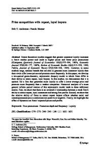
It could also be the case, however, that firm 1 is uniformly less aggressive in sequential than in simultaneous bidding. Example 2 Hansen (1988) proved that in the case of simultaneous competition, the symmetric equilibrium bidding function is more aggressive in a variable-quantity first-price auction than the analogous bidding function in a fixed-quantity first-price auction. Let φF (b) be the equilibrium inverse bidding function in the first-price auction with a fixed quantity. Then, φF (b) < φ0 (b) for all b < c. −1
e 1−c Suppose F (c) = 1− 1−e −1) and Q(p) = 2−p. Figure 1 depicts φF (b) (the continuous −1 (e
line) and φ1 (b) (the broken line). Since φ1 (b) < φF (b) for all b < c, it follows that φ1 (b) < φ0 (b) for all b < c. 8
Notice as well that −Q(b)/Q0 (b) has to be bounded below for the pM (c) to be well defined. Then, it has to
be true that γ(c) = 0.
8
1 0,9 0,8 0,7 0,6 0,5 0,4 0,3 0,2 0,1 0 0,4
0,5
0,6
0,7
0,8
0,9
1
F igure 1
4
Welfare and efficiency
We shift our attention now to the firms’ expected profits, buyer surplus and efficiency at the equilibria of the simultaneous and the sequential case. There are at least two interesting questions to pose. The first question focuses exclusively on the case of sequential competition, and follows the lines proposed by the literature on first- vs. second-mover advantages mentioned in the introduction. It sounds intuitively plausible that the second mover fares better than the first mover. We would like to ascertain whether that is true in our model or not. A second issue links sequential with simultaneous competition. It would be interesting to know how expected seller profits, buyer surplus and efficiency compare between the equilibria corresponding to both timings. We deal with these two questions in what follows. Is there a second-mover advantage in the sequential game? The next proposition provides a positive answer. Proposition 2 Let Ui1 (c) be firm i’s interim expected profit in the sequential game, i = 1, 2. Then, U21 (c) > U11 (c) for all c < c. Proof. For any c, U21 (c)
=
Z
c
φ1 (c)
[b1 (s) − c]Q(b1 (s))f (s)ds 9
Then, since φ1 (c) < c for any c < c, Z c 1 [b1 (s) − c]Q(b1 (s))f (s)ds > [b1 (c) − c]Q(b1 (c))[1 − F (c)] U2 (c) > c
where the last inequality follows from the fact that (b − c)Q(b) is increasing in b and b1 (c) is
increasing. Since
U11 (c) = [b1 (c) − c]Q(b1 (c))[1 − F (b1 (c))] the result follows. Let us now compare the equilibria of the simultaneous and the sequential game in terms of buyer and bidder welfare and efficiency. This comparison could be relevant for any model that tried to endogenize the game’s timing, as stated above. Let Ui0 (c) be firm i’s interim expected utility when its cost is c in the case of simultaneous competition. As for the first mover, it is straightforward that it is U11 (c) < U10 (c) for all c < c. Indeed, the situation firm 1 faces in the sequential case is the same it would face in the simultaneous case if firm 2 bid its own cost. Since at the equilibrium of the simultaneous game firm 2 bids above its cost, it has to be true that firm 1 is better off. The comparison, however, is not as clear in the case of the second mover. If it is the case that firm 1 is not more aggressive in the sequential game than it is in the simultaneous game for any cost level (i.e. if b1 (c) ≥ b0 (c) for all c), then U21 (c) > U20 (c) follows: not only does firm
2 hold the advantage of moving second, but it also faces a less aggressive rival. In other words,
for every cost realization (c1 , c2 ), (i) if firm 2 wins in the simultaneous game, it wins as well in the sequential game, and it does so at a higher price; and (ii) it is possible that firm 2 loses in the simultaneous game and wins in the sequential game. Still, as we have shown, there is a whole class of cases where b1 (c) < b0 (c) for all c < c. Hence, we cannot rule out the possibility that firm 1 becomes so much more aggressive in the sequential game that firm 2 ends up being worse off.9 Comparing expected buyer surplus and efficiency between the two games presents similar complications. Note that both equilibria lead to market inefficiency: for all cost pairs (c1 , c2 ), the final price is higher than min{c1 , c2 }. But finding out which game generates a higher buyer
surplus or more efficiency hinges upon how prices compare in both cases. Just as above, if
b1 (c) ≥ b0 (c) for all c it has to be the case that, for all cost pairs, the corresponding price is higher in the sequential game. Then, expected buyer surplus is lower when competition is sequential, 9
Still, we cannot provide an example where that happens.
10
and simultaneous competition is more efficient. But it may be the case that b1 (c) < b0 (c) for all c < c, so that, for some cost pairs, the corresponding price is lower in the sequential game than in the simultaneous one. Then, we cannot make a general assertion. Proposition 3 shows that if H(b) is convex, however, prices are stochastically lower with simultaneous price competition. Note that the class of cases the proposition refers to includes all those that satisfy the sufficient conditions specified in Proposition 1. Proposition 3 If H(b) is convex, then expected buyer surplus and expected total surplus are lower in the simultaneous than in the sequential game. Proof. Hansen (1988) showed that, under our assumptions, both expected buyer surplus and expected total surplus are lower in a second-price than in a first-price auction. Then, it suffices to show that both surpluses are lower in our simultaneous game than in a second-price auction. To do so, let GSP A (b) be the cumulative distribution function of the equilibrium price in the case of a variable-quantity, second-price auction, and let G1 (b) be its analog in our sequential game. We will show that GSP A (b) > G1 (b) for all c < c. Given this first-order stochastic dominance relation, and the fact that buyer and total surplus are decreasing in price, the result follows. Since in a second-price auction each firm bids its own cost, GSP A (b) = (F (b))2 . In addition, G1 (b) = F (φ1 (b)). For all b ∈ (c, b1 (0)), we have GSP A (b) > G1 (b) = 0. Clearly, then, if both distributions cross at some bb < c, it has to be the case that GSP A0 (bb) < G10 (bb). But, since GSP A (c) = G1 (c) = 1, this implies that, for some eb ∈ (bb, c), we must have GSP A0 (eb) = G10 (eb) and GSP A (eb) < G1 (eb). Hence,
or
G10 (eb) GSP A0 (eb) < G1 (eb) GSP A (eb)
f 0 (φ1 (eb))φ10 (eb) 2f (eb) < F (φ1 (eb)) F (eb) As F (c) is logconcave, f (b)/F (b) is decreasing. Then, the last inequality can only hold if φ10 (eb) < 2. However, from (2), φ10 (b) = 1 − H 0 (b). It can be easily checked that H 0 (c) = −1. Given that H(b) is decreasing and convex, φ10 (eb) > 2, a contradiction.
5
Conclusion
We have examined a simple model with two possible interpretations: (i) Bertrand competition when firms’ costs are private information, and (ii) first-price procurement auctions with endogenous quantity. By comparing the equilibria that follow from simultaneous and sequential 11
price-quoting, we conclude that moving first may lead a firm to bid more or less aggressively that it would in a simultaneous game. The second mover, however, holds an advantage. Moreover, shifting from simultaneous to sequential competition has, under some conditions, negative consequences for buyer surplus and efficiency. If we take the oligopoly interpretation of our games, and along the lines of the literature that examines the endogenous timing of moves in symmetric-information cases, it would then be interesting to add a first stage where firms strategically determine the order of moves when there is incomplete information. This, however, remains to be done.
References [1] Amir, R. and I. Grilo (1999), “Stackelberg versus Cournot Equilibrium,” Games and Economic Behavior, 26, 1-21. [2] Amir, R. and A. Stepanova (2006), “Second-Mover Advantage and Price Leadership in Bertrand Duopoly,” Games and Economic Behavior, 55, 1-20. [3] Anderson, S. and M. Engers (1992), “Stackelberg vs. Cournot Oligopoly Equilibrium,” International Journal of Industrial Organization, 10, 127-135. [4] Arozamena, L. and F. Weinschelbaum (2006a), “The Effect of Corruption on Bidding Behavior in First-Price Auctions,” mimeo, Universidad Torcuato Di Tella and Universidad de San Andrés. [5] Arozamena, L. and F. Weinschelbaum (2006b), “A Note on the Suboptimality of Rightof-First-Refusal Clauses,” Economics Bulletin, 4, No.24, 1-5. [6] Bagnoli, M. and T. Bergstrom (2005), “Log-concave Probability and its Applications,” Economic Theory, 26, 445-469. [7] Bagwell, K (1995), “Commitment and Observability in Games,” Games and Economic Behavior, 8, 271-280. [8] Bikhchandani, S., S. Lippman and R. Ryan (2005), “On the Right-of-First-Refusal,” Advances in Theoretical Economics, 1, No.1, Article 4.
12
[9] Burguet, R. and M. Perry (2005), “Preferred Suppliers and Vertical Integration in Auction Markets,” mimeo, Institut d’Analisi Economica and Rutgers University. [10] Dastidar, K.G., (2004), “On Stackelberg Games in a Homogeneous Product Market,” European Economic Review, 48, 549-562. [11] Dowrick, S. (1986), “von Stackelberg and Cournot Duopoly: Choosing Roles,” RAND Journal of Economics, 17, 251-260. [12] Gal-Or, E. (1985), “First Mover and Second Mover Advantages,” International Economic Review, 26, 649-653. [13] Gal-Or, E. (1986), “Information Transmission - Cournot and Bertrand Equilibria,” Review of Economic Studies, 53, 85-92. [14] Gal-Or, E. (1987), “First-Mover Disadvantages with Private Information,” Review of Economic Studies, 54, 279-292. [15] Grosskopf, B. and A. Roth (forthcoming), “If You Are Offered the Right of First Refusal, Should You Accept? An Investigation of Contract Design,” Games and Economic Behavior. [16] Hamilton, J. and S. Slutsky (1990), “Endogenous Timing in Duopoly Games: Stackelberg or Cournot Equilibria,” Games and Economic Behavior, 2, 29-46. [17] Hansen, R. (1988), “Auctions with Endogenous Quantity,” RAND Journal of Economics, 19, 44-58. [18] Hurkens S. and E. van Damme (1999), “Endogenous Stackelberg Leadership,” Games and Economic Behavior, 28, 105-129. [19] Lofaro, A. (2002), “On the Efficiency of Bertrand and Cournot Competition under Incomplete Information,” European Journal of Political Economy, 18, 561-578. [20] Maggi, G. (1999), “The Value of Commitment with Imperfect Observability and Private Information,” RAND Journal of Economics, 30, 555-574. [21] Mailath, G. (1993), “Endogenous Sequencing of Firm Decisions,” Journal of Economic Theory, 59, 169—182. 13
[22] Maskin, E. and J. Riley (1984), “Optimal Auctions with Risk Averse Buyers,” Econometrica, 52, 1473-1518. [23] Shi, X. (2006), “Optimal Auctions with Endogenous Quantity,” mimeo, Yale University. [24] Spulber, D. (1995), “Bertrand Competition When Rivals’ Costs Are Unknown,” Journal of Industrial Economics, 43, 1-11.
14