Single-Cell Based Random Neural Network for Deep

Single-Cell Based Random Neural Network for Deep Learning Yonghua Yin and Erol Gelenbe FIEEE Intelligent Systems and Networks Group Electrical & Electronic Engineering Department, Imperial College, London SW7 2AZ, UK Abstract—Recent work demonstrated the value of multi clusters of spiking Random Neural Networks (RNN) with dense soma-to-soma interactions in deep learning. In this paper we go back to the original simpler structure and we investigate the power of single RNN cells for deep learning. First, we consider three approaches with the single cells, twin cells and multi-cell clusters. This first part shows that RNNs with only positive parameter can conduct convolution operations similar to those of the convolutional neural network. We then develop a multi-layer architecture of single cell RNNs (MLSRNN), and show that this architecture achieves comparable or better classification at lower computation cost than conventional deeplearning methods.

I. I NTRODUCTION The Random Neural Network (RNN) was developed to mimic the behaviour of biological neurons in the brain [1], [2] and its generalisations [3]. Applications of the RNN have focused on its recurrent structure and learning capabilities [4] especially in image processing [5], [6], as well as in recent work [7]–[12]. While early work [13] investigated the links between conventional optimisation and the RNN, much more recently [14] the RNN was connected to deep learning [15]–[18] and the extreme learning machine (ELM) concept [19], [20]. In particular, we proposed a multi-layer architecture composed of multiple clusters of recurrent RNNs with dense soma-to-soma interactions to implement autoencoders with a training procedure [14], [21] that is significantly faster than existing deep-learning tools. This paper investigates the value of single RNN cells for deep learning. Specifically we show that, with only positive parameters, the RNN implements convolution operations similar to convolutional neural networks [16], [22], [23]. Our work examines single-cell, twin-cell and cluster approaches that model the positive and negative parts of a convolution kernel as the arrival rates of excitatory and inhibitory spikes to receptive cells. We also investigate the relationship between the RNN and ReLU activation [24] and suggest an approximate ReLU-activated convolution operation. Also, we build a multi-layer architecture composed of single-cell RNNs (MLSRNN), different from the densecluster based architecture in [14], [21], in which the final layer is an ELM rather than RNN cells and clusters. The computational complexity of the MLSRNN is much lower than the dense model [14], [21], and it can be generalized to handle multi-channel datasets.

Numerical results regarding multi-channel classification datasets, with an image and two time-series, show that the single-cell based RNN is effective and that it is arguably the most efficient among five different deep-learning approaches. II. R ECURRENT R ANDOM N EURAL N ETWORK An arbitrary cell in the Random Neural Networks (RNN) can receive excitatory or inhibitory spikes from external sources, in which case they arrive according to independent Poisson processes. Excitatory or inhibitory spikes can also arrive from other cells to a given cell, in which case they arrive when the sending cell fires, which happens only if that cell’s input state is positive (i.e. the neuron is excited) and inter-firing intervals from the same neuron v are exponentially distributed random variables with rate rv ≥ 0. Since the firing times depend on the internal state of the sending cell, the arrival process of cells from other cells is not in general Poisson. From the preceding assumptions it was proved in [1], [2], [25] that for an arbitrary N cell RNN, which may or may not be recurrent (i.e. containing feedback loops), the probability in steady-state that any cell h, located anywhere in the network, is excited is given by the expression: PN + λ+ v=1 qv rv pvh h + qh = min( , 1), (1) P N − rh + λ− v=1 qv rv pvh h + − for h = 1, ... , N , where p+ vh , pvh are the probabilities that cell v may send excitatory or inhibitory spikes to cell h, − and λ+ h , λh are the external arrival rates of excitatory and inhibitory spikes to cell h. For notation ease, we also use + − − wvh = rv p+ vh and wvh = rv pvh as excitatory and inhibitory connecting weights. Note that min(a, b) is a element-wise operation whose output is the smaller one between a and b. In [25], it was shown that the system of N non-linear equations (1) have a solution which is unique.

III. C ONVOLUTION O PERATION WITH RNN: T WO A PPROACHES In this and the next sections, we show that, though with only positive parameters, the RNN is capable of conducting convolution operators that produce similar effects to those in conventional convolutional neural networks [16], [23], by three approaches, which is denoted as O = conv(I, W ) with O, I and W being the output, input and convolution kernel.

I

I1

Excitatory and Inhibitory Spikes

O

O

I

Excitatory Spikes Inhibitory Spikes

I2

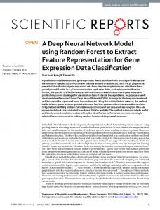
Fig. 1.

Excitatory and Inhibitory Spikes

An RNN convolution operation with single-cell approach. Fig. 2.

A. Single-Cell Approach We construct a type of RNN cells and present the procedure for conducting convolution operations using these cells. An RNN cell receives excitatory and inhibitory spikes from external cells denoted by x+ and x− , and it also receives excitatory spikes from outside world denoted by λ+ . The firing rate of the cell is r. Then, based on (1), the probability in the steady state that this cell is activated is λ + + x+ , 1), q = min( r + x−

(2)

For notation ease, we define φ(x+ , x− ) = min((λ + x+ )/(r + x− ), 1) and use φ(·) as a term-byterm function for vectors and matrices. First, we normalize the convolution kernel to satisfy the RNN probability constraint via W ← W/(sum(|W |)/r). Second, we spilt it as W + = max(W, 0) ≥ 0 and W − = max(−W, 0) ≥ 0 to avoid negativity (another RNN probability constraint). Operation sum(a) produces the summations of all elements in a and max(a, b) produces the larger element between a and b. Then, the RNN convolution operation can be conducted using RNN cells (2) O = φ(conv(I, W + ), conv(I, W − ))

(3)

O = φ(conv(I, W − ), conv(I, W + )),

(4)

or +

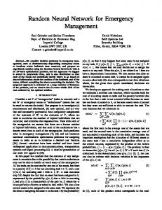
where λ and r are usually set as the same value for simplicity. The convolution operation with single cells is shown schematically in Figure 1. B. Twin-Cell Approach This approach is also based on RNN cells (2). From (2), we have φ(0, I)|λ+ =1,r=1 = 1 − φ(I, I)|λ+ =0,r=1 . To satisfy the RNN probability constraints, we first normalize the convolution kernel via W ← W/sum(|W |) and split it into W + = max(W, 0) ≥ 0 and W − = max(−W, 0) ≥ 0. As seen from Figure 2, input I passes through a twincell array and produces I1 = φ(0, I)|λ+ =1,r=1 and I2 = φ(I, I)|λ+ =0,r=1 . The receptive cell are quasi-linear cells [26] (called the LRNN-E cell) that receive excitatory spikes from outside world with rate λ+ = 1 − sum(W − ). We can also normalize the input to receptive cells via W + ← W + /max(O0 ) and W − ← W − /max(O0 ) to reduce the number of cells that are saturated [26], where O0 =

An RNN convolution operation with twin-cell approach.

conv(I1 , W + ) + conv(I2 , W − ) + 1 − sum(W − ). Then, the RNN convolution operation can be conducted as O = min(conv(I1 , W + )+conv(I2 , W − )+1−sum(W − ), 1). (5) IV. C ONVOLUTION O PERATION WITH RNN: A C LUSTER A PPROACH This approach is based on a type of multi-cell cluster that approximates the rectified linear unit (ReLU) that has been widely-used in the deep-learning area [16], [24]. The cluster is constituted by the LRNN-E cell [26] and another different quasi-linear RNN cell that is deduced from a firstorder approximation of the RNN (1). A. First-Order Approximation of the RNN The formula (1) lends itself to various approximations such as the first order approximation: PN PN + − λ+ λ− v=1 qv rv pvh v=1 qv rv pvh h + h + qh ≈ [1 − ], (6) rh rh PN − provided that rh >> λ− v=1 qv rv pvh . The proof of (6) h + is given in the Appendix. + − − + − Let wvh = rv p+ vh = 0, wvh = rv pvh , λh = 1, λh = 0, rh = 1 and rv = 1. Note these settings do not offend the Pthat N condition rh >> λ− + q p− 1 >> v=1 v rvP h vh , which becomes PN PN N − − − w q . Since r = 1, then w = p v v v=1 vh h=1 vh h=1 vh ≤ 1. The first-order approximation (6) can be rewritten as: qh =

1 PN

1+ PN

− v=1 wvh qv

≈ min(1 −

N X

− wvh qv , 1),(7)

v=1

PN − subjecting to ≤ 1 and 1 >> v=1 wvh qv . PN P N − − Since qv ≤ 1, we have v=1 wvh qv ≤ Pv=1 wvh , and N − we then could loose the condition 1 >> v=1 wvh qv to PN − 1 >> v=1 wvh , which is independent of the cell states. This simplified RNN cell receiving inhibitory spikes is quasi linear, and thus we could call it a LRNN-I cell. − h=1 wvh

B. Relationship between RNN and ReLU Based on the LRNN-E cell [26] and LRNN-I cell (7), we investigate the relationship between the RNN and the ReLU activation function [16], [24] and show that a cluster of the LRNN-I and LRNN-E cells produces approximately the ReLU activation.

1) ReLU Activation: We consider a single unit with ReLU activation. Suppose the input to the unit is a nonnegative 1×V vector X = [x1,v ] in the range [0, 1], and the connecting weights is a V × 1 vector W = [wv,1 ] whose elements can be both positive and negative. Then, the output of this unit is described by ReLU(XW ) = max(0, XW ). Let W + = + − [wv,1 ] = max(0, W ) and W − = [wv,1 ] = − min(0, W ). It + − is clearly that W ≥ 0, W ≥ 0, W = W + − W − and ReLU(XW ) = max(0, XW + − XW − ). 2) A Cluster of the LRNN-I and LRNN-E Cells: First, we import X into a LRNN-E cell with connecting weights W − :

I

O

Excitatory Spikes

Excitatory and Inhibitory Spikes

Fig. 3.

An RNN convolution operation with cluster approach.

q1 = min(XW − , 1). Let us suppose XW − ≤ 1. Then, q1 = XW − . In the meantime, we import X into a LRNN-I cell with W +: 1 ≈ min(1 − XW + , 1). q2 = 1 + XW + Based PV on+ (7), the condition of this approximation is that v=1 wv,1 1 (i.e., XW < 0) is removed by the LRNN-E cell. We have q3 = ϕ(XW + , XW − ) ≈ 1 − ReLU(XW ),

(8)

where, for notation ease, we define the activation of this cluster as ϕ(x+ , x− ) = min(1/(1 + x+ ) + x− , 1) and use ϕ(·) as a term-by-term function for vectors and matrices. The conditions for the P approximation in (8) are XW − ≤ 1 (that V − can be loosed as v=1 wv,1 = sum(W − ) ≤ 1 if X ≤ 1) PV + and v=1 wv,1 = sum(W + ) > a. Then, we can approximate qh in a neighbourhood φ = r as:

∂qh qh ≈ qh |φ=a + |φ=a (φ − a) ∂φ P PN N + + λ+ λ+ v=1 qv rv pvh v=1 qv rv pvh h + h + = − (φ − a) rh + a (rh + φ)2 PN PN λ+ + v=1 qv rv p+ λ+ + v=1 qv rv p+ vh vh ≈ h − h (φ − a) rh rh2 PN + λ+ φ a v=1 qv rv pvh h + ≈ (1 − + ) rh rh rh

≈

λ+ h +

PN

+ v=1 qv rv pvh

rh

(1 −

φ ). rh

Then, qh ≈

λ+ h

+

PN

+ v=1 qv rv pvh

rh

(1 −

λ− h

+

PN

− v=1 qv rv pvh

rh

).

R EFERENCES [1] E. Gelenbe, “Random neural networks with negative and positive signals and product form solution,” Neural computation, vol. 1, no. 4, pp. 502–510, 1989. [2] ——, “Stability of the random neural network model,” Neural computation, vol. 2, no. 2, pp. 239–247, 1990. [3] ——, “G-networks: a unifying model for neural and queueing networks,” Annals of Operations Research, vol. 48, no. 5, pp. 433–461, 1994. [4] ——, “Learning in the recurrent random neural network,” Neural Computation, vol. 5, no. 1, pp. 154–164, 1993. [5] C. Cramer, E. Gelenbe, and H. Bakircloglu, “Low bit-rate video compression with neural networks and temporal subsampling,” Proceedings of the IEEE, vol. 84, no. 10, pp. 1529–1543, 1996. [6] E. Gelenbe and C. Cramer, “Oscillatory corticothalamic response to somatosensory input,” Biosystems, vol. 48, no. 1, pp. 67–75, 1998. [7] S. Mohamed and G. Rubino, “A study of real-time packet video quality using random neural networks,” IEEE Transactions on Circuits and Systems for Video Technology, vol. 12, no. 12, pp. 1071–1083, 2002. [8] G. Rubino and M. Varela, “A new approach for the prediction of endto-end performance of multimedia streams,” in Quantitative Evaluation of Systems, 2004. QEST 2004. Proceedings. First International Conference on the. IEEE, 2004, pp. 110–119. [9] M. Mart´ınez, A. Mor´on, F. Robledo, P. Rodr´ıguez-Bocca, H. Cancela, and G. Rubino, “A grasp algorithm using rnn for solving dynamics in a p2p live video streaming network,” in Hybrid Intelligent Systems, 2008. HIS’08. Eighth International Conference on. IEEE, 2008, pp. 447–452. [10] H. Larijani and K. Radhakrishnan, “Voice quality in voip networks based on random neural networks,” in Networks (ICN), 2010 Ninth International Conference on. IEEE, 2010, pp. 89–92. [11] K. Radhakrishnan and H. Larijani, “Evaluating perceived voice quality on packet networks using different random neural network architectures,” Performance Evaluation, vol. 68, no. 4, pp. 347–360, 2011. [12] T. Ghalut and H. Larijani, “Non-intrusive method for video quality prediction over lte using random neural networks (rnn),” in Communication Systems, Networks & Digital Signal Processing (CSNDSP), 2014 9th International Symposium on. IEEE, 2014, pp. 519–524. [13] E. Gelenbe and S. Timotheou, “Random neural networks with synchronized interactions,” Neural Computation, vol. 20, no. 9, pp. 2308–2324, 2008. [14] E. Gelenbe and Y. Yin, “Deep learning with random neural networks,” 2016 International Joint Conference on Neural Networks (IJCNN), pp. 1633–1638, 2016. [15] G. E. Hinton and R. R. Salakhutdinov, “Reducing the dimensionality of data with neural networks,” Science, vol. 313, no. 5786, pp. 504–507, 2006. [16] Y. LeCun, Y. Bengio, and G. Hinton, “Deep learning,” Nature, vol. 521, no. 7553, pp. 436–444, 2015. [17] R. Raina, A. Madhavan, and A. Ng, “Large-scale deep unsupervised learning using graphics processors,” in Proc. 26th Int. Conf. on Machine Learning. ACM, 2009, pp. 873–880. [18] D. C. Ciresan, U. Meier, L. M. Gambardella, and J. Schmidhuber, “Deep big simple neural nets for handwritten digit recognition,” Neural Computation, vol. 22, pp. 3207–3220, 2010. [19] L. L. C. Kasun, H. Zhou, and G.-B. Huang, “Representational learning with extreme learning machine for big data,” IEEE Intelligent Systems, vol. 28, no. 6, pp. 31–34, 2013. [20] J. Tang, C. Deng, and G.-B. Huang, “Extreme learning machine for multilayer perceptron,” to appear in IEEE Transactions on Neurla Networks and Learning Systems, May 2015. [21] Y. Yin and E. Gelenbe, “Deep Learning in Multi-Layer Architectures of Dense Nuclei,” ArXiv e-prints, Sep. 2016. [22] Y. LeCun, L. Bottou, Y. Bengio, and P. Haffner, “Gradient-based learning applied to document recognition,” Proceedings of the IEEE, vol. 86, no. 11, pp. 2278–2324, 1998. [23] J. T. Springenberg, A. Dosovitskiy, T. Brox, and M. Riedmiller, “Striving for simplicity: The all convolutional net,” arXiv preprint arXiv:1412.6806, 2014.

[24] X. Glorot, A. Bordes, and Y. Bengio, “Deep sparse rectifier neural networks.” in Aistats, vol. 15, no. 106, 2011, p. 275. [25] E. Gelenbe, “Learning in the recurrent random neural network,” Neural Computation, vol. 5, pp. 154–164, 1993. [26] Y. Yin and E. Gelenbe, “Nonnegative autoencoder with simplified random neural network,” ArXiv e-prints, Sep. 2016. [27] Theano Development Team, “Theano: A Python framework for fast computation of mathematical expressions,” arXiv eprints, vol. abs/1605.02688, May 2016. [Online]. Available: http://arxiv.org/abs/1605.02688 [28] I. MODULE, “Googlenet: Going deeper with convolutions.” [29] A. Vedaldi and K. Lenc, “Matconvnet – convolutional neural networks for matlab,” in Proceeding of the ACM Int. Conf. on Multimedia, 2015. [30] O. Russakovsky, J. Deng, H. Su, J. Krause, S. Satheesh, S. Ma, Z. Huang, A. Karpathy, A. Khosla, M. Bernstein, A. C. Berg, and L. Fei-Fei, “ImageNet Large Scale Visual Recognition Challenge,” International Journal of Computer Vision (IJCV), vol. 115, no. 3, pp. 211–252, 2015. [31] A. Beck and M. Teboulle, “A fast iterative shrinkage-thresholding algorithm for linear inverse problems,” SIAM journal on imaging sciences, vol. 2, no. 1, pp. 183–202, 2009. [32] Y. Zhang, Y. Yin, D. Guo, X. Yu, and L. Xiao, “Cross-validation based weights and structure determination of chebyshev-polynomial neural networks for pattern classification,” Pattern Recognition, vol. 47, no. 10, pp. 3414–3428, 2014. [33] Y. Yin and Y. Zhang, “Weights and structure determination of chebyshev-polynomial neural networks for pattern classification,” Software, vol. 11, p. 048, 2012. [34] Y. Zhang, Y. Yin, X. Yu, D. Guo, and L. Xiao, “Pruning-included weights and structure determination of 2-input neuronet using chebyshev polynomials of class 1,” in Intelligent Control and Automation (WCICA), 2012 10th World Congress on. IEEE, 2012, pp. 700–705. [35] F. Chollet, “Keras,” https://github.com/fchollet/keras, 2015. [36] Y. LeCun, F. J. Huang, and L. Bottou, “Learning methods for generic object recognition with invariance to pose and lighting,” in Computer Vision and Pattern Recognition, 2004. CVPR 2004. Proceedings of the 2004 IEEE Computer Society Conference on, vol. 2. IEEE, 2004, pp. II–97–104. [37] K. Altun, B. Barshan, and O. Tunc¸el, “Comparative study on classifying human activities with miniature inertial and magnetic sensors,” Pattern Recognition, vol. 43, no. 10, pp. 3605–3620, 2010. [38] B. Barshan and M. C. Y¨uksek, “Recognizing daily and sports activities in two open source machine learning environments using body-worn sensor units,” The Computer Journal, vol. 57, no. 11, pp. 1649–1667, 2014. [39] K. Altun and B. Barshan, “Human activity recognition using inertial/magnetic sensor units,” in International Workshop on Human Behavior Understanding. Springer, 2010, pp. 38–51. [40] J. Fonollosa, L. Fern´andez, A. Guti´errez-G´alvez, R. Huerta, and S. Marco, “Calibration transfer and drift counteraction in chemical sensor arrays using direct standardization,” Sensors and Actuators B: Chemical, 2016. [41] N. Srivastava, G. E. Hinton, A. Krizhevsky, I. Sutskever, and R. Salakhutdinov, “Dropout: a simple way to prevent neural networks from overfitting.” Journal of Machine Learning Research, vol. 15, no. 1, pp. 1929–1958, 2014.