Email: {kurkoski,yama,kingo}@ice.uec.ac.jp ... paper coding and lossy source coding. ... coding of low-density parity-check codes, where the messages are real ...
ISIT 2009, Seoul, Korea, June 28 - July 3, 2009
Single-Gaussian Messages and Noise Thresholds for Decoding Low-Density Lattice Codes Brian M. Kurkoski, Kazuhiko Yamaguchi and Kingo Kobayashi Dept. of Information and Computer Engineering University of Electro-Communications Chofu, Tokyo, Japan Email: {kurkoski,yama,kingo}@ice.uec.ac.jp
Abstract—A new method for decoding low-density lattice codes is given, wherein the belief-propagation decoder messages are single Gaussian functions. Since the message can be represented by two numbers, a mean and a variance, the complexity of this decoder is lower than previous decoders, which either quantized the mixture, or used a mixture of Gaussians. The computational complexity at the check node is also lower. The performance of various code designs, under single-Gaussian decoding, is evaluated by noise thresholds. In particular, the proposed decoding algorithm has noise threshold within 0.1 dB of the quantized-message decoder, which is considerably more complex.
I. I NTRODUCTION Lattices play an important role in various information theoretic problems, including coding for the AWGN channel, dirtypaper coding and lossy source coding. Low-density lattice codes (LDLC) are lattices defined by a sparse inverse generator matrix, decoded using a belief-propagation algorithm [1]. Sommer, Feder and Shalvi proposed this lattice construction, described its belief-propagation decoder, and gave extensive convergence analysis. With decoding complexity which is linear in the dimension, it is possible to decode LDLC lattices with dimension of 106 . When used on the unconstrained-power AWGN channel, a noise threshold appeared within 0.6 dB of capacity. These characteristics make LDLC lattices a suitable candidate for these information theoretic problems. In belief-propagation decoding of LDLC lattices, the messages are mixtures of Gaussian functions; contrast this with decoding of low-density parity-check codes, where the messages are real numbers. The Gaussian-mixture nature of the decoder messages is appealing is for a decoder implementation. LDLC lattices and their belief-propagation decoder are reviewed in Section II. Unfortunately, the number of Gaussians in the mixture grows doubly exponentially in the number of iterations, and a naive implementation using Gaussians is infeasible. Currently, there are two methods to represent this message in the decoder. One is to quantize the function; fine quantization is required, as many as 1024 points [1]. The main source of complexity is a discrete-Fourier transform taken at the check node. The other is to approximate the mixture of Gaussians using a smaller 0 This
research was partially supported by the Ministry of Education, Science, Sports and Culture; Grant-in-Aid for Scientific Research (C) number 19560371.
978-1-4244-4313-0/09/$25.00 ©2009 IEEE
number of Gaussians, via a mixture-reduction algorithm; the messages can be accurately represented by a maximum of 30 numbers (the mean, variance and mixing coefficient of 10 Gaussians) [2]. Here, the main source of complexity is the Gaussian mixture-reduction algorithm. This paper proposes a decoder for LDLC lattices where the messages consist of a single Gaussian. A single Gaussian is represented by just two parameters, the mean and variance. This is an improvement in memory storage, compared to previous methods. The check node and variable node functions are also simplified. The check node finds the convolution of the incoming messages. However, since the inputs are single Gaussians, and the convolution of Gaussians is another Gaussian, the check node function only sums the means and variances of the inputs. The variable node finds the product of the incoming messages. The product of Gaussians is also another Gaussian. Since there are multiple Gaussians (corresponding to the multiple integer solutions in lattice decoding), an approximation is introduced. Moment matching, also called method of moments, is used to approximate this mixture by a single Gaussian. This method is distinct from the aforementioned mixture-reduction algorithm, which allows for multiple Gaussians in the output. In Section III, the singleGaussian belief-propagation decoding algorithm is described. The penalty for using a simplified decoder is performance loss. Comparisons are performed by finding noise thresholds, evaluated using a Monte Carlo approach. In particular, we find that the single-Gaussian decoder comes within 0.1 dB of the performance of a much more complex decoder. Noise thresholds are also found for a variety of LDLC codes. This is described in Section IV. Section V is the conclusion. It was observed during the Monte Carlo simulations that the means and variances had several interesting properties, for example, the message mean, was itself, a Gaussian random variable. These properties are described in the Appendix. II. LDLC L ATTICE BACKGROUND A. Lattices and Unconstrained Power AWGN System A lattice is a regular infinite array of points in Rn . An n-dimensional lattice Λ is defined by an n-by-n generator matrix G. The lattice consists of the discrete set of points
734
ISIT 2009, Seoul, Korea, June 28 - July 3, 2009
x = (x1 , x2 , . . . , xn ) ∈ Rn with x = Gb,
(1)
where b = (b1 , . . . , bn ) is the set of all possible integer vectors, bi ∈ Z. Lattices are linear, in the sense that x1 + x2 ∈ Λ if x1 and x2 are lattice points. We consider the unconstrained power system, as was used by Sommer, et al. Let the codeword x be an arbitrary point of the lattice Λ. This codeword is transmitted over an AWGN channel, where noise zi with noise variance σ 2 is added to each code symbol. Then the received sequence y = {y1 , y2 , . . . , yn } is: yi
= xi + zi , i = 1, 2, . . . , n.
/2 0 0 1 /2 0 0 −1 0
0 −1 0 0 − 1/2 0 0 1 /2
0 0 −1 − 1/2 1 /2 0 0 0
0 0 1 /2 0 1 0 0 − 1/2 (a)
1 0 0 0 0 1 /2 1 /2 0
0 1 /2 − 1/2 0 0 1 0 0
0 1 /2 0 1 0 0 1 /2 0
− 1/2 0 0 0 0 − 1/2 0 −1
(2)
b as the estimated A maximum-likelihood decoder selects x b. codeword, and a decoder error is declared if x 6= x The capacity of this channel is the highest noise power σ 2 at which a maximum-likelihood decoder can recover the transmitted lattice point with error probability as low as desired. In the limit that n becomes asymptotically large, there exist lattices which satisfy this condition if and only if [3]: | det(G)|2/n . (3) 2πe In the above | det(G)| is the volume of the Voronoi region, which is the measure of lattice density. σ2
1
(b) Fig. 1. (a) An inverse generator matrix H for LDLC codes, with det H = −1.505. (b) The corresponding bipartite graph.
≤
B. LDLC Lattices A low-density lattice code is a dimension n lattice with a non-singular generator matrix G, for which H = G−1 is sparse with constant row and column weight d. For a given V = | det G| and a parameter w, the inverse generator H is designed as follows. Let h = [1, w, w, . . . , w, 0, . . . , 0]
(4)
be a row vector with a single one, followed by d − 1 w’s (w ≥ 0), followed by n − d zeros. The matrix H can be written as permutations πi of h, followed by a random sign change Si , followed by scaling by k > 0: S1 · π1 (h) S2 · π2 (h) H = k (5) .. . Sn · πn (h) such that the permutations result in H having exactly one 1 in each column, and exactly d − 1 w’s in each column. The sign-change matrix Si is a square, diagonal matrix, where the diagonal entries are +1 or -1 with probability one-half. Then, k is selected to normalize the determinant to V : S1 · π1 (h) S2 · π2 (h) −1/n 1/n k = V . (6) det .. . Sn · πn (h) An example of an n = 8, d = 3 LDLC with w = 1/2 and V = −1.505 is shown in Fig. 1-(a). The corresponding
bipartite graph is shown in Fig. 1, where circles represent variable nodes (rows of H) and squares represent checks (columns of H). The above is a special case of the standard LDLC constructions, which are characterized by a parameter α ≥ 0. Belief-propagation decoding of LDLC lattices will converge exponentially fast if and only if α ≤ 1 [1, Theorem 1]. For the construction considered here, α = (d − 1)w2 , or, r α w= . (7) (d − 1) Thus, in this paper, LDLC lattice constructions characterized by the parameters n, d and α are considered. For convenience, it is assumed that |V | = 1. C. LDLC Belief-Propagation Decoder To establish notation, the LDLC belief-propagation decoder [1] is described. The bipartite-graph contains nd edges, so there are nd variable-to-check messages qk (z), and nd checkto-variable messages rk (z), k = 1, 2, . . . , nd. And, a Gaussian with mean m and variance v is denoted as: (z−m)2 1 N (z; m, v) = √ (8) e− 2v . 2πv On an AWGN channel with variance σ 2 , node i has the channel� output yi , and the initial message is qk (z) = N z; yi , σ 2 for all edges k connected to variable node i. 1) Check Node: The input and output messages are qk (z) and rk (z), respectively, for k = 1, 2, . . . , d. The associated edge labels from H are h1 , . . . , hd . Without loss of generality, the output rd (z) is found by first computing the convolution: z � z � z � red (z) = q1 ∗ q2 ∗ · · · ∗ qd−1 , (9) h1 h2 hd−1
735
ISIT 2009, Seoul, Korea, June 28 - July 3, 2009
III. S INGLE G AUSSIAN B ELIEF -P ROPAGATION D ECODER q!1 (z)
h1
q1 (z)
q2 (z)
xa
q!2
h2
xb
q!3
r!4 (z), r!4! (z) h4
h3
q3 (z)
r4 (z)
xc
(a)
The previous section described belief-propagation decoding of LDLC lattices in general terms. For AWGN channels, the messages r(z) and q(z) are always mixtures of an impractically large number of Gaussians. Prior approaches either quantized the message [1] or used another Gaussian mixture approximation. This section describes a special case of the Gaussianmixture decoder: all messages will be approximated by a single Gaussian function. The key step is performing the approximation, and here moment matching (or method of moments) is used. Because the target is a single-Gaussian message, moment matching is optimal, in the sense of minimizing the divergence between the original Gaussian mixture and the single Gaussian approximation. 3) Check node: The input to the check node q1 (z), . . . , qd−1 (z) are single Gaussians with mean mi /22 and variance vi
xd
Messages for Those Variables
Variables xa
xb
xc
qi (z)
ha xa
hb xb
hc xc
q!i (z)
ha xa + hb xb + hc xc
1
b − (h1 xa + h2 xb + h3 xc ), b = · · · , −1, 0, 1, · · ·
rkoski, Yamaguchi, Kobayashi. University of Electro-Communications, Tokyo
r!4! (z)
1 h4
xd = b − (h1 xa + h2 xb + h3 xc ) h4
r!4 (z)
r4 (z)
(b) Fig. 2.
= N (z; mi , vi ) .
qi (z)
Since the convolution of Gaussians is a Gaussian, the result of the shaping operation can be written as:
Check node (a) bipartite graph, (b) sample messages.
red0 (z) Kurkoski, Yamaguchi, Kobayashi. University of Electro-Communications, Tokyo
followed by a stretching operation,
(15)
where,
/22
= red (−hd z).
(10)
∞ X
=
rek0 (z −
b=−∞
b ). hd
(11)
A bipartite graph labeled with messages is illustrated in Fig. 2-(a). Samples of messages illustrating the unstretch, convolution, extension and stretch operations are in Fig. 2-(b). 2) Variable Node: Without loss of generality, consider the variable node inputs rek (z), k = 1, . . . , d − 1 and output qd (z). � The channel message is a single Gaussian y(z) = N z; y, σ 2 . At variable node i, take the product of incoming messages, and normalize: Product: = N z; yi , σ 2
�
d−1 Y
ri (z).
1X hk mk , and hd k=1 Pd−1 2 k=1 hk vk . h2d
m = −
The last check node operation is a shift-and-repeat extension operation for the unknown integer b,
qbd (z)
= N (z; m, v) ,
d−1
red0 (z)
rk (z)
(14)
v
=
(16) (17)
Variable Node The input to the variable node is 0 re10 (z), . . . , red−1 (z) are single Gaussians with mean mi and variance vi , rei0 (z)
= N (z; mi , vi ) .
(18)
and h1 , . . . , hd−1 are the associated edge coefficients. Now, r(z), after shift and repeat, is a mixture of Gaussians, but it is internal to the variable node: � X � b N z; rk (z) = (19) + mk , vk . hk b∈B
The variable node function (12) can be re-written as: ! � �� , qd (z) ≈ rd−1 (z) · · · r2 (z) · r1 (z) · y(z)
(12)
i=1
Normalize: qd (z)
=
qbd (z) . qb (z)dz −∞ d
R∞
(13)
The check-to-variable messages are periodic, but the channel message is not. Thus, the variable-to-check node is not periodic, and most of its energy is concentrated within a fixed interval.
where ≈ is written to indicate that the moment matching approximation will be used. The above can be written as a recursion on ai (z), initialized with a1 (z) = y(z),
(20)
and for i = 1, 2, . . . , d − 1:
736
ai+1 (z) ≈ ri (z) · ai (z),
(21)
ISIT 2009, Seoul, Korea, June 28 - July 3, 2009 3.5
r!(z) 1 h
!1
0 (a)
3
1
ai (z)
0 (b)
Noise Threshold (Distance from Capacity, dB)
!1
r(z)
0 (c)
2.5
2
1.5
1
0.5
1
0 0.1
r(z) · ai (z) !1
d=3 d=4 d=5 d=6 d=7 Full−complexity
0.2
0.3
0.4 0.5 0.6 α (LDLC design parameter)
1
0.9
and variance v as (22): ai+1 (z)
0 (d)
0.8
Fig. 4. Noise thresholds, measured in distance from capacity, for various LDLC lattices with parameters d and α. “Full complexity” at 0.6 dB refers to the SNR of the waterfall for a dimension 106 lattice with d = 7 [1], decoding using a quantized implementation.
ai+1 (z) !1
0.7
= N (z; m, v) ,
which is given by: X c0 (b)m0 (b) and m =
1
(26)
(27)
b∈B
v
Fig. 3. Steps at the variable node. (a) Single Gaussian input from check node. (b) Repeated message and single Gaussian for recursion. (c) Product. (d) Moment matching.
where the output is qd (z) = ad (z). Again, ≈ shows that the moment matching approximation will be used at each step in the recursion. Let ai (z) be a single Gaussian with mean ma and variance va , and let r(z) be a shift-and-repeated Gaussian, with mean mc , variance vc and period 1/h. The product two Gaussians is Gaussian, so the right-hand side of (21) is the Gaussian mixture: X c0 (b)N (z; m0 (b), v 0 ) ri (z) · ai (z) = (22) b∈B
with mc ma � vc va b + + vc + va vc h vc va vc va 0 v = vc + va 1 (b/h + mc − ma )2 � c0 (b) ∝ exp − , 2 vc + va
m0 (b)
=
(23) (24) (25)
where a proportionality constant is chosen so c0 (b) sum to 1. Since moment matching is being performed, the output ai+1 (z) is the single Gaussian which has the same mean m
= v0 +
X
X �2 � c0 (b)m0 (b) .(28) c0 (b) m02 (b) −
b∈B
b∈B
An example of the various functions involved in the onestep recursion are shown in Fig. 3. This figure is exaggerated; usually r(z) · ai (z) is well-approximated by only one or two Gaussians. IV. N OISE T HRESHOLDS Noise thresholds are used to characterize the performance of LDLC lattices and the belief-propagation decoder. The noise threshold is the lowest SNR for which belief-propagation decoding of an asymptotically large dimension lattice converges. Finite-dimensional lattices are not evaluated in this paper; using noise thresholds simplifies evaluation by eliminating the lattice dimension n as a parameter. Density evolution is the term used for a class of methods used to find the noise thresholds. True density evolution can be used for binary low-density parity-check codes on the AWGN channel, because the decoder messages are scalars, and the density (or distribution), can be discretized [4]. However, Monte Carlo density evolution is used for other types of codes, such as non-binary low-density parity-check codes, because the message consists of multiple parameters, and true density evolution is impractically complex [5]. The belief-propagation decoder for LDLC lattices presented here uses two numbers for each message, a mean and a variance. Performing true density evolution, in the sense of
737
ISIT 2009, Seoul, Korea, June 28 - July 3, 2009
binary low-density party-check codes, would require a joint distribution in two variables. While not intractable, is nonetheless computationally demanding. Instead, Monte Carlo density evolution will be used, as is done for non-binary low-density parity check codes, as follows. At each half iteration samples for Ns = 105 nodes were randomly drawn from an input pool, and then placed in an output pool. The pool has two types of messages to distinguish the edges with label 1 from those with label w. The output pool becomes the input pool for the next half iteration, and this procedure repeats until convergence was detected. The mean of the variable-to-check message v for the wlabeled edge was used to check convergence. When the mean (over all Ns samples) fell below 0.001, within 50 iterations, then convergence was declared. For the lattice construction considered in this paper, h = [1, w, · · · , w, 0, · · · , 0], and with w < 1, the power is suitably normalized, since such lattices have 1/| det H| = VΛ → 1 as the dimension becomes large. These thresholds, obtained using the single-Gaussian decoder, are shown in Fig. 4 for LDLC lattices with various parameters d and α. The noise thresholds improve for increasing α and d. In most cases, increasing α above 0.7 had little or no benefit for improving the threshold. Also, the noise threshold gradually improves for increasing d, however there appears to be marginal benefit for increasing beyond d = 7, as was found by Sommer, et al. Since the complexity is proportional to d, increasing d beyond this value is not a promising means to improve the threshold. Note that the d = 7, α = 0.7 ∼ 0.9 noise threshold looses about 0.1 dB with respect to a high-dimension lattice (with similar parameters d and α) decoded using quantized beliefpropagation implementation. This 0.1 dB penalty appears to be a small price to pay for the benefit of a much simpler decoder. V. C ONCLUSION LDLC lattices are powerful coding lattices, and have potential application for use on AWGN channels, dirty paper coding and lossy source coding. This paper introduced a decoder for LDLC lattices which uses a single Gaussian as message, and we demonstrated that this decoder has a noise threshold within 0.1 dB of a much more complex decoder. Monte Carlo density evolution was used to find thresholds, and a natural extension of this work is to use true density evolution. True density evolution operates faster than the Monte Carlo methods, so this could then be used to design of capacity-approaching irregular LDLC lattices. A PPENDIX When the messages are treated as random variables, three properties of interest emerge. Under a tree-like assumption, the messages r(z) are independent, and the object of interest is the probability distribution on this message, and in particular, since r(z) is represented by two scalars, mc and vc , it is of interest to find properties of the distributions of mc and vc . Similarly, properties of q(z), specifically the distributions of mq and vq are of interest.
The three properties can be found by making a simplifying assumption. Assumption 1 The one-step variable node function (27) and (28) can be well approximated by: va vc ma mc � m = + (29) va + vc va vc va vc v = . (30) va + vc This approximation drops the dependence on b, which is surprising. While this simplification is not precise, it allows us to derive the following three properties, which appeared to hold approximately during Monte Carlo density evolution. Property 1 The variances vc and vq are constants. On the first iteration, the messages q(z) and r(z) are Gaussians with variance equal to the channel variance σ 2 . On successive iterations, (30) has no dependence on the means, so the variances remain constant. In the Monte Carlo simulations, the variances were observed not to be constant, but tightly distributed. Property 2 The means mc and mq are zero-mean Gaussian random variables. Since the channel value y is a zero-mean Gaussian, both q(z) and r(z) on the first iteration are also zero-mean Gaussians. On successive iterations, since the variances are constant, we observe from (29) that the new mean is a scaled sum of means. The distribution of a sum is the convolution, and the distributions are Gaussian, so the convolution of Gaussians is Gaussian. Inductively, the Gaussian property of the means is maintained as iterations progress. In the Monte Carlo simulations, the means appeared Gaussian. Property 3 On any given iteration, the variance of mc is equal to the constant vc , likewise the variance of mq is equal to the constant vq . This property also holds on the first iteration. To show that it holds inductively, assume that Var ma = va and Var mc = vc and then find the variance of (29) as: � v v ma mc �� va vc a c Var + = , (31) va + vc va vc va + vc which is the same as (30). This property was also observed empirically during Monte Carlo simulations. For all of these properties, similar inductive arguments can be made for the function at the check node. R EFERENCES [1] N. Sommer, M. Feder, and O. Shalvi, “Low-density lattice codes,” IEEE Transactions on Information Theory, vol. 54, pp. 1561–1585, April 2008. [2] B. Kurkoski and J. Dauwels, “Message-passing decoding of lattices using gaussian mixtures,” in Proceedings of IEEE International Symposium on Information Theory, (Toronto, Canada), IEEE, July 2008. [3] G. Poltyrev, “On coding without restrictions for the AWGN channel,” IEEE Transactions on Information Theory, vol. 40, pp. 409–417, March 1994. [4] T. J. Richardson and R. L. Urbanke, “The capacity of low-density parity check codes under message-passing decoding,” IEEE Transactions on Information Theory, vol. 47, pp. 599–618, February 2001. [5] M. C. Davey, Error-correction using low-density parity-check codes. PhD thesis, University of Cambridge, 1999.
738