Proceedings of the International MultiConference of Engineers and Computer Scientists 2008 Vol II IMECS 2008, 19-21 March, 2008, Hong Kong
Single Point FDM Algorithm Development for Points One Unit from a Metal Surface David Edwards, Jr., Member, IAENG Abstract— High precision multi region FDM calculations require the use of accurate algorithms not only for general mesh points of the net but also for points one unit from a metal surface. This paper corrects and extends a theory previously presented by including the possibility of a non constant tangential flux near the surface. Comparison of these results with the general meshpoint algorithm for the two tube lens shows that the two have similar precisions. Index Terms—high precision, FDM, algorithms, electrostatic potential. I.
INTRODUCTION
The finite difference method is one of the standard methods [1]-[4] for solving an electrostatic boundary value problem having Direclet boundary conditions (potential known on a closed boundary). In this method a typically square net is placed over the geometry and then relaxed. The relaxation process consists of stepping through the points of the net and at each point finding its potential value using the surrounding meshpoints. The use of multiregions in the FDM calculations has allowed high precision to be obtained for the relaxation process. The algorithms used in these calculations are typically of order 8 or larger and require the use of potentials from the outer ring of mesh points surrounding the central point when evaluating the potential at the central point. Fig 1 shows the 24 mesh points surrounding b0, the central point. In this figure the darkened points represent the meshpoints required for the order 10 algorithm. For mesh points one unit from a metal surface the use of points in the outer ring requires determining the potential at points within the metal. Although it may seem obvious that the potential of those points would be the potential of the metal itself, this replacement simply doesn’t work. This due is to the requirement [5] that there be a power series representation of the potential in the neighborhood of the central mesh point which in turn requires that the potential be analytic in a neighborhood of the central mesh point which contains all of the requisite meshpoints. Since the neighborhood of a point one unit from a metal surface containing all required mesh points also contains the surface and at the surface the potential has a singularity in its normal derivative, a power series representation of the potential is not valid at points within the metal element. In view of above, calculations prior to ~2007 [5], [6] developed algorithms for points one unit from a metal surface which did not require points within the metal itself. As suggested in [7], a departure from a compact set of mesh points can lead to a significant degradation of the algorithmic precision. (A compact set of meshpoints would be the set for
Manuscript received December 6, 2007 Author is a member of the IJL Research Center, Newark, VT 05871 USA, 802 467 1177
[email protected]
ISBN: 978-988-17012-1-3
which the sum of the distances of the mesh points from the central point is minimal)
meshpoint labeling r b12
b13
b14
b15
b16
b11
b2
b3
b4
b17
b10
b1
b0
b5
b18
b9
b8
b7
b6
b19
b24
b23
b22
b21
b20
z
Fig. 1. Seen are the 24 mesh points surrounding the central point. For a point b0 one unit below a metal surface the points b13, b14, and b15 are virtual points(see text). The filled circles represent the points used in the order 10 general mesh point algorithm.
In 2007 [7] a theory was developed which reportedly overcame the above difficulty and allowed the potentials from points within the metal to be determined by a type of reflection of the value of the symmetric physical point. In this theory, the physical potential (it can be considered as the potential one would measure with a voltmeter) was replaced by a function called the analytic continuation of the physical potential. This function is analytic everywhere and matches the physical potential on and within the geometry. The points of the analytic continuation function located within the metal elements are called virtual points. In the above reference algorithms for computing the values for the virtual points from the adjacent physical points were derived. The theory was tested in two test geometries of that reference and showed that algorithmic precisions of points one unit below a metal surface were equivalent to those of general mesh points in the mesh (those points having the two surrounding rings entirely within the geometry and not within any element). As [7] was the first work in the area of high precision multiregion FDM, the theory along with the high precision reference nets were simultaneously developed. The test geometries mentioned above were used to test all of the algorithms and considered to have sufficient field configurations for adequate testing. In a continuation of the development of high precision reference nets for other geometries, a high precision net for the two tube geometry was developed and is shown in Fig.2.
IMECS 2008
Proceedings of the International MultiConference of Engineers and Computer Scientists 2008 Vol II IMECS 2008, 19-21 March, 2008, Hong Kong The algorithmic calculations for this geometry behaved in a manner similar to the test geometries of [7] for all algorithms with the exception of algorithms for points one unit from a metal surface. For these points there was in fact a considerable degradation of the algorithmic precision from the precisions of general mesh point algorithms.
two tube lens gap/dia = 0.1 158 162 40
V=0
V = 10
20
19 18
The essential assumption of the theory developed in [7] was that in a small pillbox surrounding the mesh point below the metal surface, the horizontal flux through the walls of the pillbox normal to the cylinder axis would be zero (or constant). The test geometries used in [7] likely satisfied this criterion resulting in the equivalence of the results with the general mesh point algorithm. A qualitative evaluation of the current high precision two tube potential data revealed that the horizontal flux immediately below the metal surface is actually not constant. Thus the assumption of the theory developed in [7] is not valid for this geometry. The present paper will extend the theory of [7] in the vicinity of a metal surface by appropriately treating a non constant horizontal flux and show that the extended theory results in the ability to use the general mesh point algorithm for mesh points one unit below a surface with similar accuracies as the general mesh point algorithm for neighboring points. II.
VIRTUAL POTENTIALS FOR POINTS ONE UNIT FROM A METAL SURFACE
0 0
160
320
Fig. 2. The two tube lens with gap/dia of .1 is shown (not to scale) together the coordinate values of various lines of the geometry. The r=19 line is one unit below the cylinder inner surface element and r=18 is one unit below it.
Fig.3 gives plots of the results for the two algorithms for this geometry. It is noted that points with r coordinate 19 are in a row one unit below the cylinder and with an r coordinate 18 the row lies one unit below this row for which the general mesh point algorithm is applicable (no required point for the algorithm lies within the metal). Seen in this figure is the loss in precision of about 3 orders of magnitude for algorithms one unit below the metal surface for grad6 ~10-8 as compared with the general mesh point algorithm for the adjacent mesh points in the row below. Thus the simple theory presented in [7] was clearly inadequate for this problem.
algorithm ic error one unit below elem ent com pared w ith error at general m esh point -10
log10(error)
-11 -12 -13 -14
sim ple reflections r = 19
-15 r = 18 general m esh pt algorithm
-16 -17 -10
-9
-8
-7
-6
-5
log10(grad6) Fig. 3. A comparison of the simple reflection algorithm of [7] with the general mesh point algorithm for the two tube lens of fig.2. Seen is that for a grad6 value of 10-8 the simple reflection algorithm looses about 3 orders of magnitude of precision.
ISBN: 978-988-17012-1-3
Since it is known that at any point strictly within the boundaries of the geometry the potential at that point satisfies Laplace’s equation and hence is an analytic function of the coordinates r and z. It is noted that Laplace’s equation is not satisfied for points on the boundary since there is a discontinuity in the derivative of the radial potential at the boundary (strictly 0 inside the metal and nonzero outside.) However one can construct an analytic function over the space which equals the physical potential within and on the boundaries of the geometry. This extended function is called the analytic continuation of the previous function and has continuous derivatives everywhere and in particular at the boundary. By construction it matches the physical potential in the physical space within the boundaries of the geometry having the value of the physical potential on the boundary. This analytically continued function could have the same algorithm for points one unit from the boundary as for a general mesh point since all points within the two rings of fig 1 are valid. For the algorithm for points one unit below the boundary the virtual points do not correspond to physical points and hence must be calculated from the physical points. It is the calculation of the values of the virtual points which will be presented below. The order 10 general mesh point algorithm has been derived in [7] and uses the darkened points of fig.1 in its evaluation of the central potential b0. Without loss of generality we will assume that the virtual point whose potential needs to be found in terms of the potential at the physical points is at radius a+1 from the axis of the cylinder and is one unit above a metal element whose radius is a. The point radius a-1 is within the geometry and is a physical point. The other situations are determined in an analogous manner. As the calculation is reasonably involved a brief sketch of the method would be perhaps useful. The potential of the virtual point at r = a+1 will be found by integrating the radial electric field between the surface at r=a and the virtual point at a+1. The radial electric field will be determined from both the radial electric field evaluated at the surface and a selection of potential expansion coefficients. The radial electric field at the surface will in turn be found in terms of the potential at a-1 which is a physical
IMECS 2008
Proceedings of the International MultiConference of Engineers and Computer Scientists 2008 Vol II IMECS 2008, 19-21 March, 2008, Hong Kong point, along with another selection of coefficients of the power series. It is noted that for a constant tangential electric field, the values of all coefficients in the above selection are zero. Thus a solution will be constructed which is a perturbation of the constant horizontal field solution. This procedure has the advantage over simply integrating the electric field found from the power series expansion of the potential at a point at the surface in that the latter gives only an approximate solution in the case of a constant horizontal field whereas the former will give the exact solution when the horizontal field is constant, i.e. it will have the correct logarithmic dependence on a. The radial electric field at a point (u, z) is in general defined by: Er(u,z) = - ∂V(r,z)/∂r evaluated at r = u, from which the following is immediately obtained: V(r2.z) – V(r1,z) = - ∫r2r1Er(u)du Letting the potential of the surface be 0, we find: a (1) V(a-1,z) = ∫ a-1Eua (2) V(a+1,z) = - ∫ aE r(u,z)du Er(r, z) must be determined for u
a and needs to be found in terms of the radial field at the surface (Er(u=a, z)). This will be done by conserving fluxes through the 4 sides of a suitably constructed pillbox shown in fig.4. (It is noted that the azimuthal flux which is normal to the surface (into the paper in fig.4a) is constant due to the assumption of axial symmetry of the geometry and is not explicitly included in the flux conservation equations.)
small pillbox below boundary F4
F1
a F2
u F3 a-1
sj u
z-h
z
delta
theta
z+h
(a) (b) Fig. 4. A small pie shaped pillbox at and below the surface of radius a shows the fluxes into and out of the pillbox. Seen in (b) is a view of the wedge along the axis along with a small ring segment used in the determination of the integral formulation of the fluxes F1, F2 normal to the hatched area.
The pillbox shown in fig.4 consists of a small wedge of length h units and having an angular spread of ∆Θ degrees. (Flux in the discussion we will always mean the normal flux.) The flux labels through the relevant surfaces are shown in this figure. It is noted that in general the flux through a surface is given by:
ISBN: 978-988-17012-1-3
F = ∫SEn(r,z)dA, where En is the electric field normal to the surface S. The calculation of the radial fluxes F4 and F3 is immediate since the area over which the integral is evaluated is arbitrarily small (of the order of h*∆Θ ) and hence the normal field can be taken to be constant over this area. The result is easily found to be: F4-F3 = (Er(a)*a-Er(u)*u)* h*∆Θ The calculation of F1 and F2 is more complex since as seen in fig.4b the area over which the fluxes must be evaluated is in general large since the r dimension varies from a-1 to a and the electric field can vary appreciably over this range of values. The appropriate integral equation may be developed by breaking the cross hatched area of fig.4b into N segments of width ∆sj, and length sj∆Θ, having an area of sj∆Θ∆sj. Since the electric field is constant over this segment the flux F1 through this segment is Ez(sj,z-h/2) sj∆Θ∆sj. The flux through the cross hatched area in fig.4b can then be found by summing all of the segment fluxes. After turning the sum to an integral in the usual manner expressions for F1 and F2 can be found. a F1 = ∫ uEz(s,z-h/2)s ds ∆Θ And a F2 = ∫ uEz(s,z+h/2)s ds ∆Θ Thus the difference between the fluxes is: a F2-F1 = ∫ u { Ez(s,z+h/2)- Ez(s,z-h/2)}/h * s ds ∆Θ h which in the limit of small h can be written: a ∫ u ∂Ez(s,z)/ ∂z * s ds ∆Θ h for ua (It is noted that in the equation (F4-F3) + (F2-F1) = 0 both F2-F1 and F4-F3 contain the factor ∆Θ h which is small and non zero and hence cancels in the conservation equation.) After conserving the fluxes through the walls of the pillbox and a small amount of algebra it is found for both u>a and u0 exactly cancel, and a series in 1/a results. The large “a” approximations are:
Including all terms in a 12th order expansion of the potential (order 13 terms neglected) the following gives the complete set of the 10 included coefficients, { c7, c12, c18, c25, c33, c42, c52, c63, c75, c88}:
(7)
(4) ∂Ez(v,z=0)/ ∂z = -(2c7v +2c12v2+2c18v3+2c25v4+2c33v5+2c42v6+2c52v7 +2c63v8+2c75v9+2c88v10) Let us define the following symbols which will help in the description of our results: a Gua (vn) = ∫ uvns ds a (5) H(vj) = ∫ a-1 Gua (vj)/u du a+1 j a J(vj) = ∫ a Gu (v )/u du Using equations 1,2,3,and 4 we find after performing all of the elementary integrations that: V(a-1) = Er(a)*a*ln(a/(a-1)) – 2c7H(v)-..-2c88H(v10) V(a+1) = Er(a)*a*ln((a+1)/a) + 2c7J(v)+..+2c88J(v10) Letting f1 = ln(a/(a-1)) and f2 = ln((a+1)/a) we can solve for the virtual potential in terms of the potential at the physical point and the expansion coefficients c7, .. c88. The results are summarized below: case 1: physical pt one unit below surface, virtual pt at a+1 V(a+1) = -V(a-1)f2/f1+corr (6) case 2: physical pt one unit above surface, virtual pt at a-1 V(a-1) = -V(a+1) f1/f2+f1/f2corr where: corr = 2c7( J(v)-f2/f1H(v) ) + .. + 2c88( J(vn)-f2/f1H(vn) ) Evaluation of H and J. H and J may be directly evaluated by elementary integrations of the equations (5) with the result: (-1)nan+2ln( a/(a-1) )/{(n+1)(n+2)} H(vn) = n+1 + (-1) ( an+1 + an/2 + .. + a/(n+1) ) /{(n+1)(n+2)} + (-1)n /(n+2)2 J(vn) = (-1)nan+2ln( (a+1)/a )/{(n+1)(n+2)} + (-1)n+1( an+1 - an/2 + ..alternating signs +- a/(n+1) ) /{(n+1)(n+2)} - (-1)n /(n+2)2 It is noted that there is an apparent an divergence in both H and J. Since in multiregion FDM “a” can reach values of 240 ~ 1012 the effect of this divergence in the above equations is immediate, obvious and limiting. It was thought that since the ln function has known expansions, a large “a” expansion of the above equations might remove the terms an and this is in fact what happened. Upon expanding the ln functions in
ISBN: 978-988-17012-1-3
H(vn) = (-1)n / {(n+1)(n+2)}* {1 + 1/( (n+3)a ) + 1/( (n+4)a2 ) + .. + 1/( (n+j)an+j-6 )} J(vn) = 1/{(n+1)(n+2)}* {1 - 1/( (n+3)a ) + 1/( (n+4)a2 )+ .. alternating signs +.. + 1/( (n+j)an+j-6 )}
Thus corr can be determined and the virtual potentials can be found in terms of the respective physical potentials. III.
CALCULATING VIRTUAL POTENTIALS FOR POINTS ONE UNIT RIGHT OR LEFT OF A METAL SURFACE
In this case the vertical surface at z may be either to the left or right of the virtual point. In either case the virtual potential can be found following procedures sketched in the above section. The result is in fact much simpler than that obtained for the horizontal surface and is given below for both cases. (8) V(z0+1) +V(z0-1) = corr corr = 4c12/(3*4) + 4c23/(5*6) +4c38/(7*8) +4c57/(9*10) + 4c80/(11*12)
For corr = 0, one has the simple reflection with sign reversal of the physical potential to virtual potential. It is noted that as mentioned in the introduction for a constant field parallel to the metal surface all of the coefficients in the selection are zero and the results of [7] are obtained as required. IV. COEFFICIENT EVALUATION Without loss of generality we restrict our example to the situation were the physical boundary is one unit above the physical point and the virtual point is one unit above the boundary. As mentioned previously the order 10 algorithm uses the darkened points of figure 1 in which the surface boundary passes through b11,b2,b3,b4,b17, and points b13,b14,and b15 are the virtual points which must be determined. The precision of the potential for these points clearly depends on the precision of the evaluation of the coefficients c7,..,c88, It should be emphasized that the coefficients are those of the power series expansion around a point on the surface itself. The coefficients can be found in an identical manner to the way that the central potential was found which was discussed in [7]. Only the physical points should be used in the coefficient evaluation. If the coefficient cj would be found by the expansion about a point on the surface then only points in and below the surface could be used. This would be a significant departure from the closest set of mesh points which as discussed in [7] has the highest precision and would result in large errors in the determination of cj’s. In view of this remark, it was decided to find the coefficients around a point immediately below the surface and then translate these coefficients into the coefficients at the surface. In this manner a set of mesh points nearer to the “closest set” can be used in the evaluation of the cj’s. To compensate for the precision degradation resulting from the departure from the closest set, order 12 algorithms were used in the coefficient determination. The transformation of coefficients one unit below the surface into the set of coefficients at the surface is straightforward and briefly described below.
IMECS 2008
Proceedings of the International MultiConference of Engineers and Computer Scientists 2008 Vol II IMECS 2008, 19-21 March, 2008, Hong Kong
W(r,z) = c0 + c1z + c2r + c3z2 + c4zr + c5r2 +.. V(r,z) = d0 + d1z + d2r +d3z2 + d4zr + d5r2+.. Note: the d’s are determined from algorithms and the c’s inferred from them. Equating W(r-1,z) with V(r,z) and setting the coefficients of rjzk to zero in the resultant equation the following equations are found relating the set of c’s to the set of d's and are enumerated for the coefficients {c3, .. , c88}. c3 = d3+d7 +d12 +d18 +d25 +d33 +d42 +d52 +d63 +d75 +d88 c7 = d7+2d12+ 3d18+ 4d25 +5d33 +6d42 +7d52 +8d63 +9d75 + 10d88 c12 = d12 +3d18+ 6d25+10d33+15d42+21d52 +28d63 +36d75 +45d88 c18 = d18+ 4d25+10d33+20d42+35d52 +56d63 +84d75+120d88 c25 = d25 +5d33+15d42+35d52 +70d63+126d75+210d88 c33 = d33 +6d42+21d52 +56d63+126d75+252d88 c42 = d42 +7d52 +28d63 +84d75+210d88 c52 = d52 + 8d63 +36d75 +120d88 c63 = d63 +9d75 +45d88 c75 = d75 +10d88 c88 = d88
It is interesting to note that the coefficients of dj‘s in the vertical columns are in fact binomial expansion coefficients. As a numerical example, using the data set of the two tube lens shown in fig.2, the coefficients cj for a point on the cylinder at r=20,z=120 are listed below: c3 c7 c12 c18 c25 c33 c42 c52 c63 c75 c88
6.4995152835614e-017 -3.0129418017510e-005 7.5323539627044e-007 5.0879925211473e-008 -9.5833188927774e-010 -3.9421070631936e-011 5.6850525669851e-013 -8.6372591936586e-015 -1.0429530261237e-014 -1.5166017528942e-015 -9.7442400560016e-017
Several features are apparent from this listing. The first is that c3 itself is very close to 0 as would be required for a point on the metal surface and is remarkable as the surface was not assumed to be an equipotential. This provides an additional validity check on both the transformation equations and the coefficient evaluations d3... d88. It should be noted that coefficients other than c3 need not be zero on the boundary since on the boundary the complete term containing these coefficients vanishes since they have rj as a factor. The second feature is that the coefficients c7 through c63 are reasonably large wrt the overall calculational precision (10-16) and since the order of magnitude of the correction term is of the order of these coefficients neglecting them can and evidently does result in the large precisional errors as seen in fig.3. V. TEST OF ALGORITHM FOR ONE UNIT BELOW ELEMENT The algorithm for a mesh point one unit below an element has been tested using the two tube lens net of fig.2 (gap/diameter = .1) as well as the zero gap lens for which there is an exact solution[8]. As mentioned above, points with r=19 are one unit below an element and require the
ISBN: 978-988-17012-1-3
determination of the virtual points b13,b14, and b15, while points with r=18 are two units below an element and all of its required points are physical points. In fig.5 the algorithmic errors for points with r=19 and r=18 for z on the half line z=0 to 160 are plotted vs the grad6 function. It may be worthwhile to emphasize that both points use the identical order 10 general mesh point algorithm, the difference being the virtual point determination for the r=19 line. Seen is that the error for the algorithm using the calculated virtual points is very similar to that of the general mesh point algorithm and offers 3 orders of magnitude improvement in the precision over the simple reflection code of [7].
error one unit below elem ent compared with error at general mesh point ref tube20 161x1281 cut-8 40 total
-10 -11
log10(error)
Let V(r,z) be the potential with origin one unit below the surface and W(r,z) be the potential with origin at the surface. Then for any r and z W(r-1,z) = V(r,z). Writing the potential expansion of W and V in terms of cj and dj respectively
-12 new code (line)
-13 -14
simple reflections r = 19
r = 18 general mesh pt
-15 -16 -17 -10
-9
-8
-7
-6
-5
log10(grad6) Fig 5. The errors for the various algorithms are compared showing the remarkable similarity in precisions of the general mesh point algorithm and the “new code” algorithm one unit below element described above.
It is noted that similar results to those of fig.5 were obtained using the Grivet net [8] mentioned above the exception that “new code” error line continued to ~10-18 rather than saturating at 10-16 seen the above figure for grad6 values less than 10-8, the improvement being due the extended precision of the exact calculation over the data from the relaxed net. VI. CONCLUSION Using the above theory, the precision of the algorithm for points one unit below an element is similar to the precision of the general mesh point algorithm. Hence these points may no longer be a significant source of contributing error to the relaxation process. In addition the rather remarkable agreement seen in the above graph is actually a confirmation of the validity of virtual potential method itself initially proposed in [7]. Although in [7] the importance of the non constant horizontal flux was not appreciated, this paper has provided the necessary framework (analytic continuation and virtual potential determination) for the correct solution to the problem. VII. NOTES OF CAUTION 1. The theory presented above is for points one unit from a vertical or horizontal element. Every part of the calculation has been checked at least once. However the only comparison with lens data is for the algorithm one unit below an element presented in this work. The other cases are expected have similar comparisons when the appropriate reference nets are constructed.
IMECS 2008
Proceedings of the International MultiConference of Engineers and Computer Scientists 2008 Vol II IMECS 2008, 19-21 March, 2008, Hong Kong 2. For every virtual point, ten 12th order coefficients must be evaluated {c7 .. c88}. Since for every calculation of the algorithm for points one unit below an element, 3 virtual points must be individually calculated 30 algorithm calculations are made per point. This multiplication of computations considerably influences the time involved in the relaxation process. However it is noted that the influence of the potential of the virtual points on calculating the central potential, b0, is only ~ 1/500. Thus the virtual points need not be evaluated on every relaxation pass. Only a slight influence on the total relax time has in fact been found using a 10% update frequency of the virtual potential values with no change in the relaxation data. 3. If the values of the virtual points are updated on every pass through the net, the relaxation process is itself unstable. Stability is brought back to the process if the new values for the virtual points are incremented by only a fraction of the change in value which has been found to be equivalent to a small update frequency as discussed above. 4. The present theory is not useful to single region FDM calculations since no gain in the after relax precisions are obtained by using algorithms much larger than 2 – 4 and these do not require points in the second ring of fig. 1. Newark, Vermont, dec 6 2007 REFERENCES [1] [2] [3] [4] [5] [6] [7] [8]
P.T. Kirstein and J.S. Hornsby, IEEE trans. Electron Devices 11, (1964) J.E. Goers, IEEE Trans. Electron Devices 12, 425(1965) D.W.O.Heddle, “Electrostatic Lens Systems”, 2nd ed., Institute of Physics Publishing, ISBN 0-7503-0697-1 ] F.H.Read, A. Adams, J.R. Soto-Montiel, J. Phys. E 4, 625(1971) D Edwards, Jr, Rev. Sci. Instrum. 54, 1,729-1735(1983) S.Natali, D.DiChiro, C.E.Kuyatt, J.Res. Nat. Bur. Stand. Sect A 76, 27(1972) D Edwards, Jr, Rev. Sci. Instrum. 78, 1,1-11(2007) P. Grivet, ”Electron Optics” London:Pergamon ,1965.
ISBN: 978-988-17012-1-3
IMECS 2008