Single View Point Omnidirectional Camera Calibration from Planar Grids

Single View Point Omnidirectional Camera Calibration from Planar Grids Christopher Mei and Patrick Rives INRIA, 2004 Route des Lucioles - BP 93, 06902 Sophia-Antipolis, Cedex - France {christopher.mei, patrick.rives}@sophia.inria.fr Abstract— This paper presents a flexible approach for calibrating omnidirectional single viewpoint sensors from planar grids. These sensors are increasingly used in robotics where accurate calibration is often a prerequisite. Current approaches in the field are either based on theoretical properties and do not take into account important factors such as misalignment or camera-lens distortion or over-parametrised which leads to minimisation problems that are difficult to solve. Recent techniques based on polynomial approximations lead to impractical calibration methods. Our model is based on an exact theoretical projection function to which we add well identified parameters to model real-world errors. This leads to a full methodology from the initialisation of the intrinsic parameters to the general calibration. We also discuss the validity of the approach for fisheye and spherical models. An implementation of the method is available as OpenSource software on the author’s Web page. We validate the approach with the calibration of parabolic, hyperbolic, folded mirror, wide-angle and spherical sensors.

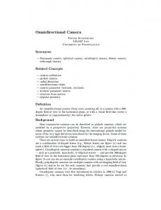
I. I NTRODUCTION Many calibration methods for omnidirectional cameras have been presented in the past few years, they differentiate themselves mainly by the type of mirror taken into account (hyperbolic or parabolic), by the projection model used (skewness, alignment errors, ...), the information that is considered as known (for example the mirror parameters) and the method used (auto-calibration, grids, ...). Non-parametric [11] approaches have also been studied. These provide interesting insights into general sensor calibration but in practice a stable calibration is difficult to obtain. Auto-calibration techniques inspired by the division model [2], [3] have lead to uncalibrated omnidirectional structure and motion [7]. However a limitation to the approach comes from the precision reported, that is well adapted to outlier rejection (RANSAC) but less satisfying for reconstruction and motion estimation. In robotics it is often a prerequisite to have accurately calibrated sensors. In the specific case of perspective cameras, methods using planar grids [14] are popular because of the simplicity of use and the accurate results they procure. This article aims at generalising this type of approach to central catadioptric sensors. We made the choice of using standard planar grids because they are commonly available and simple to make. In [10], the authors propose a method relying on a polynomial approximation of the projection function. With this model, initial values of the projection function are difficult to obtain so the user has to select each point of the calibration grid independently for the calibration. We will show that by using an exact model to which we add small errors, only four

Mirror : Rw,Tw

a,b (or p)

Mirror : a,b (or p) Rw,Tw

F

F

R1,T1

Grid

Grid

telecentric lens distortion

Optical System (lens(es))

R2,T2

camera lens distortion

radial and tangential distortion

Camera

principal point, skewness

Fig. 1. Complete calibration parameters

Camera principal point, skewness

Fig. 2.

Simplified parameters

points need to be selected for each calibration grid. The parameters that appear in the proposed model can also be easily interpreted in terms of the optical quality of the sensor. Figure 1 presents the different parameters that could be taken into account for example in the case of a parabolic mirror with a telecentric lens. Gonzalez-Barbosa [5] describes a calibration method to estimate all of these parameters. However too many parameters make the equations difficult to minimise because of the numerous local minima, the need for a lot of data and the numerical instability introduced into the Jacobian. We decided to reduce the number of parameters by making the assumption that the errors due to the assembly of the system are small (Fig. 2). To obtain a calibration that stays valid for all central catadioptric systems, we use the unified model of BarretoGeyer [4], [1] and justify its validity for fisheye and spherical sensors (Section II). In Section III we describe the different steps of the projection model. Section IV discusses the initialisation of the parameters and Section V the calibration steps. Finally, we validate the approach on real data. II. U NIFIED PROJECTION MODEL For sake of completeness, we present here a slightly modified version of the projection model of Geyer and Barreto [4], [1] (Fig. 4). We choose the axis convention depicted in Figure 3. The projection of 3D points can be done in the following steps (the values for (ξ, η) are detailed Table I and the mirror equations are given in Table II) :

TABLE II M IRROR EQUATIONS

p

πp

K

Camera z

Parabola

mu

y

Hyperbola

x

πmu X

z

Xs

y x

1

(z+ d )2 2 a2 d (z+ 2 )2 a2

−

y2 b2 y2 b2

=1

Ellipse + + =1 Plane z = − d2 With ’−’ for a hyperbola and ’+’ an ellipse : q for p p a = 1/2( d2 + 4p2 ± 2p) b = p( d2 + 4p2 ± 2p)

m

ym


zs


Fp

Fig. 4.

ξ ys


xs Cp


Unified image formation

a) Validity for fish-eye lenses: In [13], the authors show that the unified projection model can approximate fisheye projections. A point imaged by perspective projection can be written: mu = (x, y, 1) = (

1) world points in the mirror frame are projected onto X the unit sphere, (X )Fm −→ (X s )Fm =
X
= (Xs , Ys , Zs ) 2) the points are then changed to a new reference frame centered in C p = (0, 0, ξ), (X s )Fm −→(X s )Fp = (Xs , Ys , Zs + ξ) 3) we then project the point onto the normalised plane, s , Ys , 1) =
(X s ) m = ( ZX s +ξ Zs +ξ 4) the final projection involves a generalised camera projection matrix K (with [f1 , f2 ] the focal length, (u0 , v0 ) the principal point and α the skew)   f1 η f1 ηα u0 f2 η v0  m = k(m) (1) p = Km =  0 0 0 1 A generalised camera projection matrix indicates we are no longer considering the sensor as a separate camera and mirror but as a global device. This is particularly important for calibration because it shows that f and η cannot be estimated independently. We will note γi = fi η. We will call lifting the calculation of the X s corresponding to a given point m (or p according to the context) : √   ξ+ 1+(1−ξ 2 )(x2 +y 2 ) x 2 2   √ x +y 2+1 2 2   )(x +y ) (2)
−1 (m) =  ξ+ 1+(1−ξ  y   √ x2 +y22 +12 2 ξ+ 1+(1−ξ )(x +y ) −ξ x2 +y 2 +1 TABLE I U NIFIED MODEL PARAMETERS

Ellipse

x2 b2 x2 b2

xm Cm


Axis conven-

Parabola Hyperbola

−

Fm
z

Convex mirror/Lens

Fig. 3. tion

p x2 + y 2 + z 2 = z + 2p

ξ 1 √

d d2 +4p2 √ d d2 +4p2

η −2p

√ −2p √

d2 +4p2 2p d2 +4p2

Planar 0 -1 d : distance between focal points 4p : latus rectum

X Y , , 1) Z Z

with ξ = 1, the same point imaged by the unified projection model gives: md = (

Y X , , 1) Z + X  Z + X 

By algebraic manipulation, we obtain the following relation:  2ρd ρu = , with ρ = m2x + m2y 1 − ρ2d which is the division model, known to approximate a large range of fisheye lenses [2]. b) Validity for spherical mirrors: A spherical sensor does not have a single viewpoint. However the results obtained by approximating it by a single projection center give satisfying results [7]. III. P ROJECTION MODEL Compared to the theoretical model, an extra distortion function is added that models the misalignment between the mirror and camera but also the telecentric distortion (ie. the deviation of the telecentric lens’s projection function from the ideal, orthographic projection model) for the parabolic case. The different transformations that intervene and the associated unknowns (Fig. 2) are: 1) rotation and translation from the grid reference frame to the mirror reference frame (extrinsic parameters), 2) reflexion on the mirror and projection of the points on the normalised plane (mirror parameter ξ), 3) application of the distortion induced by the lens(es) (distortion parameters), 4) projection in the image with the generalised camera projection matrix (camera intrinsic parameters). Had we considered the system as a separate mirror and camera, the distortion would have been applied before the collineation induced by η. The effect is however the same as it consists only in a change of variable.

A. Extrinsic parameters The extrinsic parameters describe the transformation between the grid frame and the camera frame. Quaternions can be used advantageously to parametrise the rotation [9]. We will note V 1 = [qw1 qw2 qw3 qw4 tw1 tw2 tw3 ] the unknowns and W the corresponding transformation. B. Mirror transformation The mirror transformation was detailed in Section II and consists simply in applying
that depends only on V 2 = [ξ]. C. Distortion We will consider two main sources of distortion [12] : imperfection of the lens shape that are modeled by radial distortion and improper lens and camera assembly (which can also include misalignment between the camera optical axis and the mirror rotational axis) that generate both radial and tangential errors. In the case of a paracatadioptric sensor, an extra telecentric lens is often added to enable the use of a perspective camera (and not orthographic). The lens has the same size as the mirror border and introduces radial errors. Five parameters can be used to model the distortion [6]. A three parameter model was chosen for the radial distortion  (with ρ = x2 + y 2 ) : L(ρ) = 1 + k1 ρ2 + k2 ρ4 + k5 ρ6

(3)

Different models can be used for the tangential distortion according to the relative importance of the alignment and angular errors. We added two extra variables to model the tangential distortion dx :

2k3 xy + k4 (ρ2 + 2x2 ) dx = (4) k3 (ρ2 + 2y 2 ) + 2k4 xy We will note D the distortion function and V 3 = [k1 k2 k3 k4 k5 ] the parameters. D. Camera model A standard pin-hole model was used for the generalised camera projection P :

γ1 (x + αy) + u0 P (X, V 4 ) = , V 4 = [α γ1 γ2 u0 v0 ] γ2 y + v0 (5) E. Final equation Let G be the composition of the different projection functions and let V be the 18 parameters : G = P ◦ D ◦ H ◦ W,

V = [V 1 V 2 V 3 V 4 ]

If the grid is composed of m points gi , with their associated image values ei , the solution to the calibration problem can be obtained by minimising the following function : 1 2 [G(V, gi ) − ei ] 2 i=1 m

F (x) =

(6)

This cost function minimises the euclidean distance between the projection of the grid and the extracted values in the image. The corresponding Jacobians can be written as :

∂H  ∂D ∂P ∂W ∂H ∂G = 1 2 ∂V ∂D 2×2 ∂H 2×2 ∂W 2×2 ∂V 2×7 ∂V 2×1 

∂P ∂D ... (7) ∂V 3 2×5 2×12 ∂V 4 2×5 2×18

IV. I NITIALISATION OF THE PARAMETERS The presented method is based on the non-linear minimisation of (6) that can be solved using for example a LevenbergMarquardt approach. For the minimisation to be successful, we need to obtain initial estimates of the parameters. By assuming that the errors from the theoretical model are small, we have k1 ≈ k2 ≈ k3 ≈ k4 ≈ k5 ≈ α ≈ 0, γ1 ≈ γ2 . We still need to find the extrinsic parameters of the grids and values for [ξ, γ, u0 , v0 ]. The image center can be used to initialise the principal point (u0 , v0 ) or it can be approximated by the center of the mirror border (assumed to be a circle). Experimentally, we will show that errors in the values of (ξ, γ) do not have a strong influence over the accuracy of the extraction process (Section VI-F). We will start by assuming ξ = 1 and show that we can estimate linearly the focal length from at least three image points that belong to a non-radial line image. Once this step applied, the extrinsic parameters can be estimated from four points of a grid of known size. A. Mirror border extraction for principal point estimation The mirror border extraction is not straight forward because of the density of information around the mirror edge. However from an estimate of the mirror radius and center given by the user (for example by clicking on an image), we can refine the values by applying the following steps : 1) remove the points that are too far from the given circle, 2) remove the points on the rays between the center and the edge points, 3) from the remaining points, create a list of possible circle centers and radii by random sampling. The median values of the lists give a robust estimate of the mirror center and radius. B. Estimation of the generalised focal length From equation (2), with ξ = 1, we obtain:   x  , f (x, y) = 1 − 1 (x2 + y 2 ) (8) y
−1 (m) ∼  2 2 f (x, y) Let p = (u, v) be a point in the image plane. Thanks to the estimate of the principal point, we can center the points and calculate a corresponding point pc = (uc , vc ). This point follows the equation on the normalised plane that depends on γ: pc = γm:   uc −1  , g(m) = γ − 1 (u2c + yc2 ) (9) vc
(m) ∼  2 2γ g(uc , vc )

If this to a line image defined by the normal  point belongs , we obtain: N = nx ny nz  2 2  c  nx uc + ny vc + a2 − b uc +v =0 2 −1 
(m) N = 0 ⇐⇒ a = γnz   b = nz γ Let us assume, we have n points p1 , p2 , ..., pn belonging to a same line image, they verify the system :   u2 +v 2 uc1 vc1 21 − c1 2 c1  .  .. .. ..  Pn×4 C4×1 = 0, with P =  . . .  ..  ucn

vcn

1 2

−

Fig. 5.

Extraction of the mirror border

2 u2cn +vcn 2

By singular value decomposition (SVD) P = USV , the least square solution is obtained from the last column of V associated to the minimal singular value. To obtain N and in particular γ from C = [c1 c2 c3 c4 ] , the following steps can be applied: 1) Calculatet = c21 + c22 + c3 c4 and check that t > 0. 2) Let d = 1/t, nx = c1 d and ny = c2 d. 3) We check that n2x + n2y > thresh (with for example thresh = 0.95) to be sure the  line image is not radial, 4) If the line is not radial, nz = 1 − n2x − n2y . 5) Finally, γ =

Fig. 6.

VI. E XPERIMENTAL RESULTS

c3 d nz

If the user selects three points or more on a line image, we can obtain an estimate of the focal length. (This process can in fact be applied to three randomly chosen points in the image to obtain an estimate of the focal length in a RANSAC fashion. This way we obtain an auto-calibration approach.) V. C ALIBRATION STEPS We suggest the following calibration steps to initialise the unknown parameters, make the associations between the grid points and their reprojection in the image and finally launch the minimisation: 1) (Optional) the user selects the mirror center and a point on the mirror border. The values are then re-estimated to obtain the center of the circle that is an estimate of the principal point (u0 , v0 ) (Fig. 5). Alternatively, the center of the image is used, 2) the user selects at least three non-radial points belonging to a line image, from here we estimate the focal length γ (Fig. 6), 3) for each calibration image, the user is then asked to select the four grid corners and the extrinsic parameters are estimated (Fig. 7), 4) the grid pattern is then reprojected and a sub-pixel accuracy extraction is performed (Fig. 8), 5) we can then perform the global minimisation. Sub-pixel point extraction: The sub-pixel point extraction for perspective cameras stays locally valid for omnidirectional sensors.

Estimation of the focal length from line image points

Our calibration approach was tested with five different configurations: parabolic, hyperbolic, folded mirror, wideangle and spherical sensors. A different camera was used each time. Care was taken to obtain points over the entire field of view for each sensor. An image was set aside during the calibration and then used to validate the intrinsic parameters. To validate our model, we need to obtain a low residual error after minimisation and a uniform distribution of the error. It is not necessary do check the error distribution over the complete image as we assume a rotational symmetry of the sensor. For each calibration, we will show the radial distribution of the fitting error with a curve representing the median value of the fitting error for different intervals of ρ. We may note that polynomial approximations are often valid only locally and badly approximate the projection around the edges. This bias will have a negative impact for

Fig. 7.

Grid corners used to initialise the extrinsic grid parameters

TABLE IV C ALIBRATION RESULTS FOR THE HYPERBOLIC SENSOR

Sub-pixel accuracy extraction of the remaining points

A. Calibration of the parabolic sensor The parabolic sensor (ξ = 1) used in this study consists of a S80 parabolic mirror from RemoteReality with a telecentric lens and a perspective camera with an image resolution of 2048 × 1016. The calibration points were obtained from 8 images of a grid of size 6 × 8 with squares of 42 mm. Table III summarises the results. After minimisation, we can see that the error is correctly distributed over the image (Fig. 9). TABLE III C ALIBRATION RESULTS FOR THE PARABOLIC SENSOR Initialisation [u0 ,v0 ] (b) = [983.65, 545.17], γ = 569, [ex ,ey ] = [1.92, 2.02] Final Values 3σ [γ1 ,γ2 ] [597.00, 594.71] [6.88, 8.05] [u0 ,v0 ] [583.31, 547.47] [3.98, 4.19] [k1 , k2 ] [-0.0857, 0.0147] [0.0078, 0.0045] [ex ,ey ] [0.17, 0.31] [0.43, 0.78] Val. [ex ,ey ] [0.18, 0.28]

Distortion: If we do not take into account the distortion during the calibration, the error increases to [0.74, 0.82] which confirms that the radial distortion function is needed to account for the error induced by the telecentric lens.

1 1

0.8 Errors in pixels

example when estimating the motion of the camera using a maximum likelihood estimation under the assumption of a Gaussian distribution of the error. The results will be summarised in a table containing the initial values after steps (0) and (1) and the results after the minimisation. [ex ,ey ] indicates the reprojection error in pixels. The values prefixed by ’Val.’ correspond to the error obtained on the image put aside for the validation. (b) means the mirror border was used to initialise the principal point.

Errors in pixels

Fig. 8.

Initialisation [u0 ,v0 ] (b) = [390.67,317.69], γ = 270, [ex ,ey ] = [1.02, 1.24] Final Values 3σ [γ1 ,γ2 ] [237.89, 237.23] [8.14, 7.89] [u0 ,v0 ] [387.21, 321.34] [ 1.69, 1.76 ] [ξ] 0.75 0.05 [k1 , k2 ] [-0.105, 0.013] [0.009, 0.001] [ex ,ey ] [0.29, 0.31] [0.73, 0.82] Val. [ex ,ey ] [0.24, 0.26]

0.6 0.4 0.2 0 200

0.8 0.6 0.4 0.2

300

400 ρ

500

600

Fig. 9. Pixel error versus distance - parabolic sensor

0 100

150

200 ρ

250

300

Fig. 10. Pixel error versus distance - hyperbolic sensor

advantage of being compact and relatively cheap to manufacture. The 10 images used had a resolution of 640 × 480, the grids had a size of 6 × 8 with squares of 30 mm. Table V summarises the results. We can see a very slight bias in the error that is stronger around the mirror border (Fig. 11). TABLE V C ALIBRATION RESULTS FOR THE FOLDED CATADIOPTRIC CAMERA

Initialisation [u0 ,v0 ] (b) = [298.53, 269.50], γ = 156.14, [ex ,ey ] = [0.368, 0.576] Final Values 3σ [γ1 ,γ2 ] [136.29, 132.80] [3.21, 3.14] [u0 ,v0 ] [299.01, 267.72] [1.47, 1.23] [ξ] 0.69 0.03 [k1 , k2 , k3 , k4 ] × [-108.03, 11.79, -2.38, 2.28] [4.67, 0.79, 0.55, 0.44] 1e−3 [ex ,ey ] [0.12, 0.18] [0.28, 0.44] Val. [ex ,ey ] [0.16, 0.15]

B. Calibration of the hyperbolic sensor In the hyperbolic case, the mirror is a HM-N15 from Accowle (Seiwapro) with a perspective camera with an image resolution of 800 × 600. 6 images of a grid of size 8 × 10 with squares of 30 mm were taken. Table IV summarises the results. After minimisation, we can see a slight bias in the error that is more important in the center of the image (Fig. 10). C. Calibration of a folded catadioptric camera Folded catadioptric sensors combine typically two mirrors and follow the single viewpoint constraint [8]. They have the

D. Calibration of a wide-angle sensor The calibration was also tested on a wide-angle sensor (∼ 70o ) on 21 images of resolution 320×240 . The grid used was the same as in the hyperbolic case. For the wide-angle sensor, there is no border so the center of the image was taken to initialise the principal point. Table VI summarises the results. As before, we can see a very slight bias towards the edges in Figure 12. The strong change in γ after minimisation is probably due to the radial distortion and the change in ξ. The value of ξ does not have a simple interpretation for wide-angle sensors.

TABLE VI C ALIBRATION RESULTS FOR THE WIDE - ANGLE SENSOR Errors in pixels

Initialisation [u0 ,v0 ] = [160, 120], γ = 448, [ex ,ey ] Final Values [γ1 ,γ2 ] [1070.84, 1079.70] [u0 ,v0 ] [166.16, 109.94] [ξ] 3.05 [k1 ] -0.74 [ex ,ey ] [0.13, 0.12] Val. [ex ,ey ] [0.07, 0.26]

0.5

= [0.73, 0.69] 3σ [0.60, 0.60] [1.56, 1.13] 0.021 0.13 [0.12, 0.13]

Errors in pixels

Errors in pixels

0.2

60

80 ρ

100

120

Pixel error versus distance - spherical sensor

TABLE VIII I NFLUENCE OF ERRORS IN (ξ, η) OVER THE POINT EXTRACTION

0.6

0.3

0.2

0 40

Fig. 13.

0.4

0.3

0.1

0.8

0.5

0.4

0.6

PROCESS 0.4

% error in (ξ, η) % of correct points

0.2

0 99.7

10 88

20 81

30 83

40 76

0.1 0

80

100 120 140 160 180 ρ

Fig. 11. Pixel error versus distance - folded catadioptric camera

0 0

50

ρ

100

150

Fig. 12. Pixel error versus distance - wide-angle sensor

process presents a certain robustness to imprecise initial values. We still managed to calibrate the sensor with an error of 40 %. C ONCLUSION

E. Calibration of a camera with a spherical mirror Finally we tested a low-quality camera consisting of a webcam in front of a spherical ball. The image resolution was of 352 × 264. 7 images were used with a similar grid as in the parabolic case. The border extraction process did not prove very efficient for this sensor so the image center was used as an initial value for the principal point. Table VII summarises the results. Figure 13 shows the radial distribution of the error. The error seems to be uniformly distributed (Fig. 13). TABLE VII C ALIBRATION RESULTS FOR THE SPHERICAL MIRROR Initialisation [u0 ,v0 ] = [184, 127], γ = 137.7, [ex ,ey ] = [0.65, 0.62] Final Values 3σ [γ1 ,γ2 ] [164.10, 161.95 ] [11.06, 10.96] [u0 ,v0 ] [185.98, 126.24] [0.49, 0.35] [ξ] 0.95 0.12 [k1 , k2 ] [-0.32, 0.066] [9.2, 7.5] ×1e−3 [ex ,ey ] [0.17, 0.15] [0.38, 0.34] Val. [ex ,ey ] [0.16, 0.15]

F. Point extraction To analyse the effect of errors on the mirror parameters over the point extraction process, we counted the amount of correctly extracted points obtained after the extrinsic parameters were estimated from four points, and the grid was reprojected followed by a sub-pixel accuracy extraction. Table VIII summarises the results for errors in (ξ, η) ranging from 0 to 40 %. These values indicate that the extraction

In this article, we presented a general calibration approach for single viewpoint omnidirectional cameras. The calibration steps are simple without the need to know the mirror parameters. We justified theoretically that the method can be used to model central catadioptric, fisheye and spherical sensors. These results were confirmed experimentally with the calibration of a wide range of sensors. R EFERENCES [1] J. P. Barreto and H. Araujo. Issues on the geometry of central catadioptric image formation. In CVPR, 2001. [2] C. Brauer-Burchardt and K. Voss. A new algorithm to correct fisheye- and strong wide-angle-lens-distortion from single images. In International Conference on Image Processing, 2001. [3] A. W. Fitzgibbon. Simultaneous linear estimation of multiple view geometry and lens distortion. In CVPR, 2001. [4] C. Geyer and K. Daniilidis. A unifying theory for central panoramic systems and practical implications. In ECCV, pages 445–461, 2000. [5] J.-J. Gonzalez-Barbosa. Vision panoramique pour la robotique mobile : st´er´eovision et localisation par indexation d’images. PhD thesis, Universit´e de Toulouse III, 2004. [6] J. Heikill¨a and O. Silv´en. A four-step camera calibration procedure with implicit image correction. In Computer Vision and Pattern Recognition, 1997. [7] B. Micusik. Two-view geometry of Omnidirectional Cameras. PhD thesis, Center for Machine Perception, Czech Technical University, 2004. [8] S. Nayar and V. Peri. Folded Catadioptric Cameras. In Panoramic Vision, pages 103–119. Apr 2001. [9] E. Salamin. Application of quaternions to computation with rotations. Stanford AI Lab., 1979. [10] A. Scaramuzza D., Martinelli and R. Siegwart. A toolbox for easy calibrating omnidirectional cameras. In IROS, 2006. [11] P. Sturm and S. Ramalingam. A generic concept for camera calibration. In ECCV, pages 1–13, 2004. [12] J. Weng, P. Cohen, and M. Herniou. Camera calibration with distortion models and accuracy evaluation. PAMI, 14(10):965–980, 1992. [13] X. Ying and Z. Hu. Can we consider central catadioptric cameras and fisheye cameras within a unified imaging model ? In ECCV, 2004. [14] Z. Zhang. Flexible camera calibration by viewing a plane from unknown orientations. In ICCV, 1999.