siss project - numerical simulation of the scour

SISS PROJECT - NUMERICAL SIMULATION OF THE SCOUR EVOLUTION AROUND THREE DIMENSIONAL SUBMERGED STRUCTURES

Michele Drago, Paolo Cherubini Snamprogetti S.p.A. FANO, ITALY

ABSTRACT A numerical procedure has been developed for the evaluation of scouring phenomena on the sea bed due to the presence of structures or unevenness. The methodology has been validated by comparison with laboratory experiments carried out under a wide range of environmental conditions and structures geometry. The results confirm the reliability of the numerical procedure as a useful tool in predicting the relevance of the bed erosion phenomena that occur when a disturbance of the flow field is introduced by a structure in an otherwise stable condition.

INTRODUCTION The stability of the sea bottom has a major impact in the design of the offshore structures, as the onset of scour phenomena may undermine the stability and the functionality of the structures. Mostly as a consequence of the lack of data, in the past years only rough approaches were available for the estimation of the scour evolution around three dimensional submerged structures and the literature reports a series of troubles experienced in the engineering practice due to the inadequate consideration paid to the problem. In the last years the problem has become even more apparent due to the increasing of the construction of underwater hydrocarbon production and transportation systems. The SISS project (Seabottom Instability around Small Structures ) aimed at developing a methodology enabling the offshore engineer to estimate the scour expected around complex three dimensional submerged structure due to the disturbance of the flow field induced by the structure itself, thus allowing to plan in the design procedure the necessary preventive and corrective actions. This scope has been pursued with an extensive series of small scale laboratory tests, the implementation of a numerical model

for the simulation of the scour evolution and a full scale field verification of the results. The numerical procedure has been developed for the evaluation of the scouring phenomena, and consequent changes in the bottom morphology, resulting when a solid structure is installed on an otherwise stable sea bottom. The numerical procedure is based on the commercial general purpose fluid dynamics code PHOENICS, which is used both for the evaluation of the flow field around the structure and the transport of suspended sediment, and on the program EVOL, specifically developed for this project, which evaluates the bed load transport and the changes in the bottom morphology. The two programmes are used in an iterative manner, until a new equilibrium condition is achieved.

THE HYDRODYNAMIC MODEL The turbulent nature of the natural flows is a driving factor of the scour evolution. Although it is generally accepted that the basic equations of fluid dynamics, namely the Navier Stokes equations, can describe even turbulence, actually this is far beyond the present computational capability, so that some kind of approximation is required when dealing with turbulent flows. In the present work the computer program PHOENICS has been used to simulate turbulent fluxes around structures laying on the sea bottom. The turbulence has been modelled adopting the - closure model, as it still represents a good compromise between accuracy and numerical simplicity, when dealing with complex turbulent flows; the flow variables are split in a constant component, which describe the macroscopic flow characteristic, and in a fluctuating one, linked to the turbulent eddies. Only the r constant part u of the velocity is solved, while the flow fluctuations effects are taken into account introducing a fictitious

viscosity, the eddy viscosity t , on account of the fact that its contribution is formally the same as the one from viscous stresses (see for ex. /1/, chap. 1). PHOENICS solves the momentum equations

  ui  u j   ui  ui 1  P     uj       t     t  xj   xi  x j    x j  xi  where

ui

is the i-th velocity component,  is the fluid density

and P is the pressure; the continuity equation

     ( u) = 0 t

    ui  t  xi  xi

 t  k   ui   ui  u j     t    x j   x j  xi    k  xi 

 t      ui   ui  u j      x   c 1 k  t  x   x   x i  j  j i  

2    c  1  k 

where the standard values /2/ of 0.09, 1.0, 1.314, 1.44 and 1.92 are usually assigned to the constant c ,  k ,   , c 1 and c 2 in the above equations respectively. The eddy viscosity, that unlike the molecular one is not a property of the flow, can be expressed as

 t  c

k2



Actually the expressions for k and are obtainedfrom the Navier Stokes equations, but so many assumptions are involved in their derivations, especially in the case of that they should be regarded as essentially empirical in nature. Following the mainstream in k - simulation /2/, in the present work, the law of the wall approach has been used to define the boundary conditions close to solid surfaces in order to avoid the zone where viscous phenomena are more important than or of the same order of the turbulent one (high Reynolds number hypothesis). From the theory of turbulent boundary layers, it is known that within a certain distance from a solid boundary a constant stress layer exists, where the profile of the time averaged flow velocity can be described by a logarithmic function as:

u( z) 

constant and zo is the bottom roughness. Within the constant stress layer rather simple expressions can be also defined for turbulent kinetic energy k and dissipation rate , namely k  u*2 c and   u*3  z where  is the Von Karman constant and z the distance from the solid surface. In k- modelling, the boundary of the computational domain close to a solid surface is defined at points which are inside the constant stress layer, which is usually assumed to extend within the range:

30

,

and the equations for turbulent kinetic energy k and its dissipation rate 

k k   ui  t  xi  xi

where u is the mean flow velocity parallel to the surface at a distance z, u* is the friction velocity, k is the Von Karman

 z  ln    z0 

u*

u*



 z  100

u*



and the formulas of the logarithmic profile defined above are used to define proper boundary values for the variables from their known values at the solid surface. PHOENICS adopts the finite volume method /5/ to discretize the general equation (1) on a three-dimensional grid: within the present work the body fitting (curvilinear) grid option of the program has been adopted for the definition of the computational meshes. This greatly increases the computational time, but allow a quite accurate geometrical description of the evolution of the bottom with the progressing of the scouring. The meshes are variable in size and they are rather small close to the solid boundaries, in order to solve accurately the high velocity gradient and calculate the stress correctly, and close to the structure, where the acceleration and the recirculation cells require a quite fine grid to be solved properly. The iterative SIMPLEST algorithm, a variant of the well known SIMPLE one /5/ is used by PHOENICS to solve the linkage between the flow variables and the non linear nature of the discrete equations.

THE MODELLING CONCENTRATION

OF

SUSPENDED

SEDIMENT

Traditionally in sediment transport studies the total transport is split into suspended load, i.e. the amount of sediment transported in suspension by the flow, and bed load, i.e. the sediment transport occurring close to the bottom. Mathematically this has the advantage that suspended load transport is described by equations formally analogue to those of the flow variables, so that the same algorithms can be used for both situations. Consequently, within the present work, a module for the evaluation of the suspended load concentration has been added to the hydrodynamics model, while the bed load contribution has been evaluated in the module of the bottom evolution. The

concentration of suspended sediment is described by the equation:

C  C  u H   H C  w  ws     C   0 t  z where C represent the fraction volume of sediment, horizontal gradient operator,

ws

H

where T     cr   cr is the stress parameter, and

is the

is the settling velocity of the

sediment, which can be evaluated as (/3/, Chap. 4):

ws 

10 d50

where s is the ratio of the sediment and water density,  is the water viscosity and d50 is the mean grain size. The sediment diffusion coefficient  is usually related to the flow eddy viscosity through the Schmidt number  t :    t  t =0.5 has been

adopted. Sediment flux from the sea bottom into the flow field can be evaluated as /4/: 1.5

 s  0.015

d 50     cr    a   cr 

ws 0. 3 D*

where the reference height a is the height of the bed load layer, which can be estimated as 10 d 50 (see /3/ Chap. 8),  is

the local bottom stress,  cr is the critical stress and

D*

is the non

dimensional sediment number:

 s  1g  D*   2    

is the

flow velocity vector close to the bottom. Hence the total sediment transport in each vertical section of the computational domain can be evaluated as Stx  S x  Qb , x and Sty  S y  Qb , y where S x and S y are the

 C  S x    uC    dz  x a H

t

 U

components of the depth integrated suspended sediment transport:

 0.01s  1gd 50 1 / 2    1 1  2   

for which in the present work a constant value

  T 1.5 U QB  0.1d 50u* 0.3 D* U 2 V 2

1/ 3

d 50

Equation (11) has been used to define the bottom boundary condition for the suspended load model.

THE MODEL OF BOTTOM EVOLUTION The computer program EVOL performs the tasks of: . evaluate the bed load transport . evaluate the sediment budget on each mesh of the bottom . evaluate the consequent increase or decrease in the bottom level and update the computational grid to account for the modifications in the bottom geometry. The bed load transport is evaluated in each computational point on the bottom with the formula /4/:

H   C  dz and S y    vC    y  a

Finally the vertical variation of the sea bottom results from the conservation of the sediment mass as:

(1  n)  s

  Zb   s  H St t

where s is the sediment density and n is the bottom porosity. As the scour hole develops, its side slopes should adapt to the flow conditions, as sediment avalanching would occur when the local slope exceed the friction angle. In principle the maximum allowable slope should depend on the local flow direction: slopes higher than the friction angle in still water could occur opposite to the flow direction, while they should result lower than the still water friction angle in the downstream and side stream directions. However the laboratory tests indicate that very weak differences in the slope angles occur within the scour hole, hence, as a first approximation, the maximum allowable slope in the model has been fixed to the friction angle in still water, which, for sand particles, can be roughly assumed equal to 30°. Hence, when locally the slope of the scour hole exceeds the maximum allowable value  max , the slope is fixed to the value of  max , interpolating the scour depth between adjacent meshes. Global conservation of the sediment mass is enforced in the process. Once that the final bottom depth has been evaluated in all the mesh points, EVOL calculate the modifications in the computational grid required to account for the new bottom morphology. In the process no additional mesh is added to the computational domain, rather the existing meshes are deformed to adapt to the new domain geometry. The condition (8) on the first grid point and the accumulation of meshes where required are preserved.

THE COMPUTATIONAL PROCEDURE FOR THE SCOUR EVOLUTION

In nature the flow field, sediment transport and scour evolution are interdependent, as the modification of the bottom morphology induces a modification in the flow field and, consequently, even in the sediment budgets. In the numerical procedure this linkage is approximated with an iterative procedure: . the flow field is evaluated with the hydrodynamic model. When the converged solution is achieved, the flow velocities and bottom stresses obtained are used to evaluate the suspended sediment concentration in equilibrium with the flow field. In the process it is assumed that no change occurs in the bottom morphology. . the total sediment budget and the depth evolution time rate at each grid point is evaluated by the EVOL program. In the process it is assumed that the fluid dynamics and the sediment transport do not change. The computation of the depth evolution is stopped when the changes become so significant that the above hypothesis results unrealistic. Hence the grid of the fluid dynamics model is updated to account for the changes in the bottom morphology. At this point a new hydrodynamic simulation is performed to evaluate the flow filed and the sediment concentration compatible with the new geometry of the computational domain. The above steps are iteratively repeated until the equilibrium condition is achieved, i.e. the distribution of the bottom stress appears uniform in the whole computational domain or everywhere the stresses are below the critical value.

VALIDATION OF THE LABORATORY TESTS

NUMERICAL

MODEL

ON

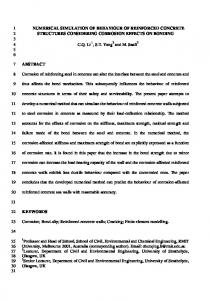
The numerical procedure for the computation of the scouring has been validated on the basis of the laboratory results obtained in erodible bed tests /6/. As boundary conditions, the current profile at the inflow section of the computational domain has been specified on the basis of laboratory measurements (fig. 1), and the associated profiles of turbulent kinetic energy k and its dissipation rate  have been defined from the velocity profiles with standard formulas available in literature /7/. At the bottom and on solid surfaces, the law of the wall with smooth hydraulic conditions has been assumed, as the condition in the experimental flume were very close to smooth ones. At the upper limit of the computational domain and at the outflow the normal derivatives have been set to zero, in steady current simulations. In wave simulations the rigid lid approximation has been used at the upper limit of the computational domain, i.e. the effect of surface elevations has been simulated with a pressure gradient established on a rigid surface. The performance of the computational procedure has been verified on the experimental data by comparing the maximum scour depth and the pattern of the scour hole. Tab. 1 lists the tests

carried out, the maximum scour depth computed and observed in laboratory tests and the percentile difference, while Tab 2 and Fig. 2 explains the meaning of the cases list in first column of tab. 1.

Fig 1

-

Vertical profiles of velocity used in the numerical model

TEST

Experimental Computed depth(cm) depth(cm)

Percentile error(%)

EBA.1.1

2.2

4.5

EBA.1.2

4.3

3.8

11.6

EBA.1.3

13.7

14.1

2.9

EBA.1.4

6.0

6.3

5.0

EBA.1.5

7.0

7.5

7.1

EBA.1.6

5.7

6.8

16.1

EBA.2.3

12.5

13.4

7.2

EBA.2.6

5.0

5.5

10.0

EBB.1.1

2.0

2.4

20.0

EBB.1.2

6.0

5.8

3.3

EBB.1.3

1.17

1.43

18.1

EBB.2.3

1.52

1.63

7.2

EBB.3.1

2.0

2.2

10.0

EBB.3.2

5.0

4.6

8.0

EBB.3.3

10.0

10.1

1.0

EBB.4.1

3.6

4.0

11.1

EBB.4.2

7.5

7.8

4.0

EBB.4.3

14.0

14.3

2.1

EBB.5.2

8.0

8.6

7.5

EBB.5.3/1

18.5

18.1

2.7

EBB.5.3/2

23.0

24.1

4.8

EBC.1.1

1.0

2.1

110.0

EBC.1.2

3.6

4.6

27.8

EBC.1.3

8.0

10.3

28.7

EBD.1.3

11.0

12.3

11.8

2.1

Tab. 1 - Comparison between numerical and experimental tests

Tab. 2 - Wave and current conditions in the different laboratory tests - U* = friction velocity; U*,c= critical value of the friction velocity; Umo=orbital significant velocity close to bottom; Kc = Keulegan Carpenter parameter (Kc = UmoTp/D - D stream wise dimension of the structure)

CONCLUSIONS Observing fig. 3 it is apparent that the percentile error on the maximum scour depth rarely exceeds 10%. The higher percentile errors are associated to the smaller scour depths: this is little surprise as in this case the absolute value of the scour depth is in the same order as the estimated precision of the computational procedure due to the spatial discretization adopted, which has been evaluated to be 0.5 cm. Large errors are associated also to the cylindrical structures, notwithstanding the facts that the computed and observed scour patterns appear rather close to each other (fig. 6). Possible reasons of the observed differences reside in the physical phenomena not properly accounted for in the numerical model. As an example the horse shoe vortex is usually regarded as a driving phenomenon for the evolution of the scour around vertical cylinders, while in the present hydrodynamic simulation this flow feature was not observed. However the overall good agreement of observed and computed scour depths indicate that the global effect of disregarded or not properly modelled phenomena should not be large. The grey zone in the histogram of fig. 3 reports the percentile errors observed in the simulations performed at the critical velocity: for these simulations, two third of the cases considered show an error smaller than 10%, so indicating that the model is more reliable at the higher flow velocities, which are also the more interesting ones in practical applications.

Environmental conditions Current test U*=1/2U*c. U*=3/4U*c. U*=U*c.

EB.A.1.1

EB.A.1.2

U*=1.7U*c. Uc/Umo=1.8 Uc/Umo=0.8 Uc/Umo=0.8 Kc=1.4 Kc=4.1 Kc=5.8

EB.A.1.3

EB.A.1.4

EB.A.1.5

EB.B.1.2

EB.A.1.6

EB.A.2.3

EB.A.2.6

EB.A.3.3

EB.A.3.6

EB.A.4.3 EB.B.1.1

Fig. 2 Description of the structures geometry and flow conditions

Wave & current tests

EB.A.4.6

EB.B.1.3

EB.B.1.4

EB.B.1.5

EB.B.2.3

EB.B.1.6 EB.B.2.6

EB.B.3.1

EB.B.3.2

EB.B.3.3

EB.B.3.4

EB.B.3.5

EB.B.3.6

EB.B.4.1

EB.B.4.2

EB.B.4.3

EB.B.4.4

EB.B.4.5

EB.B.4.6

EB.B.5.1

EB.B.5.2

EB.B.5.3

EB.C.1.1

EB.C.1.2

EB.C.1.3

EB.C.1.4

EB.C.1.5

EB.C.1.6

EB.D.1.3

EB.B.5.7

Some comparisons of the computed and experimental scour patterns are shown in fig. 4 - 5 - 6 for the steady current simulations, and in fig. 7 for current plus waves simulations. The figures show a good agreement either as concern the extension of the scour zone and the maximum scour depths. The scour pattern is usually caught by the numerical simulation in front and at the side of the structure, while the agreement deteriorates in the zone behind the structures, where the computed scour extension appears underestimated. However, the overall agreement appear rather good, and this is particularly significant as regard the reliability of the procedure, as the comparison has been performed for different structure shapes

(cube, prism, cylinder), different undisturbed flow conditions (U  U cr , U  3 / 4 U cr ) and different angle of incidence of the flow on prismatic structures, without significant differences in the performance of the model. Some observations should be done as concern the cases with waves plus current (cases EBA.1.4-5-6, EBA.2.6). Although even in these situations the agreement between computed and observed scour is good, at least as concern the maximum scour depth, it should be noted that the computational procedure has been developed mainly for steady current situations and there are good reasons, such as the approximation of time varying conditions with successive equilibrium steady states, the adoption of a logarithmic profile close to the bottom etc., to consider it not really suitable for waves plus current flow conditions. Hence, in waves plus current conditions, the model has not been used to the same extent as in steady current ones.

Cases number

Numerical - experimental difference (%) 10 5 0