function and using an optimization algorithm to select the best window length, or (ii) using all ... A common task in stream mining is to detect and monitor frequent .... We are interested in the performance of two statistics: the cost of the optimal.
Size Matters: Finding the Most Informative Set of Window Lengths Jefrey Lijffijt a , Panagiotis Papapetrou b
ab
, and Kai Puolam¨aki
a
a Department of Information and Computer Science, Aalto University, Finland?? Department of Computer Science and Information Systems, Birkbeck, University of London, UK
Abstract. Event sequences often contain continuous variability at different levels. In other words, their properties and characteristics change at different rates, concurrently. For example, the sales of a product may slowly become more frequent over a period of several weeks, but there may be interesting variation within a week at the same time. To provide an accurate and robust “view” of such multi-level structural behavior, one needs to determine the appropriate levels of granularity for analyzing the underlying sequence. We introduce the novel problem of finding the best set of window lengths for analyzing discrete event sequences. We define suitable criteria for choosing window lengths and propose an efficient method to solve the problem. We give examples of tasks that demonstrate the applicability of the problem and present extensive experiments on both synthetic data and real data from two domains: text and DNA. We find that the optimal sets of window lengths themselves can provide new insight into the data, e.g., the burstiness of events affects the optimal window lengths for measuring the event frequencies. Keywords: event sequence, window length, clustering, exploratory data mining
1
Introduction
Many sequences involve slowly changing properties, mixed with faster changing properties. For example, the sales of a product may slowly become more frequent over a period of several weeks, but there may be interesting variation throughout a week at the same time. To provide an accurate and robust “view” of such multi-level structural behavior, one needs to determine the appropriate levels of granularity for analyzing the underlying sequence. Sliding windows are frequently employed in several sequence analysis tasks, such as mining frequent episodes [25], discovering poly-regions in biological sequences [29], finding biological or time-series motifs [6, 7], analysis of electroencephalogram (EEG) sequences [30], or in linguistic analysis of documents [3]. A major problem is that such methods are often parametrized by a user-defined ??
This work was supported by the Finnish Centre of Excellence for Algorithmic Data Analysis Research (ALGODAN).
2
Size Matters: Finding the Most Informative Set of Window Lengths 0.2 Window size: 1562 Window size: 6250
Relative frequency
0.15
0.1
0.05
0 0
1
2
3
4
5 6 Starting position in X
7
8
9
10 4
x 10
Fig. 1. Frequency change of an event in a sequence X of length 100,000. We use two sliding windows of lengths 1562 and 6250. The generative process for this sequence is described in Section 5.2. We observe that the two window lengths describe two different views of the data.
window length and it can be unclear how to choose the appropriate window length that guarantees optimal execution of the task at hand. This problem can be avoided by either (i) defining an appropriate objective function and using an optimization algorithm to select the best window length, or (ii) using all possible window lengths at the same time. The first approach has, on one hand, the limitation that a single window length may leave out important information that would be discovered when using other window lengths. On the other hand, studying all window lengths does not have this deficiency, however, it may be challenging to analyze the large amount of information. The method proposed in this paper is to use a small set of window lengths that together provide as much information as possible about the underlying data. We demonstrate that for many sequences an optimal balance between the two previous problems can be obtained. Example. The frequency of an event in a sequence may show variation at different levels. Figure 1 shows an example of the relative frequency of an event over time, which is computed using two incremental sliding windows of lengths 1562 and 6250. The generative process for this sequence is described in Section 5.2. We observe that each window length tells us a different “story” about the frequency of the event. In other words, each window describes a different view of the data: the longer window suggests a “smoothly” increasing frequency throughout the sequence, while the shorter window captures a periodic behavior in the event frequency. Contribution. In this paper we introduce the novel problem of finding a good set of window lengths for analyzing discrete sequences. We define suitable criteria and an efficient method for choosing window lengths, and give examples of tasks that demonstrate the applicability of the problem to different domains. We perform extensive experiments on real data from two application domains: text books and DNA sequences. We find that the scales of the occurrence pat-
Size Matters: Finding the Most Informative Set of Window Lengths
3
terns of various events (e.g., word types or DNA segments) vary significantly, and that the optimal scales can provide useful new insight into the data. Finally, we conduct an evaluation of optimal window lengths for random data to compare the empirical results with.
2
Related Work
String and text mining. Sliding windows have been used extensively in string mining. Indexing methods for string matching based on n-grams [21], i.e., subsequences of length n, employ sliding windows of fixed or variable length to create dictionaries and speed-up approximate string search in large collections of texts. Determining the appropriate window length is always a challenge, as small window lengths result in higher recall but large index structures. In text mining, looking at different linguistic dimensions of text results in extracting different “views” of the underlying text structure [3]. One way to quantify these views is by using sliding windows. Recently, an interactive text analysis tool1 has been developed for exploring the effect of window length on three commonly used linguistic measures: type-token ratio2 , proportion of hapax legomena, and average word length. However, the window length is user-defined. Bioinformatics. Several sliding window approaches have been proposed for analyzing large genomes and genetic associations. Two groups of methods exist in the literature that are characterized by fixed-length and variable-length sliding windows [4, 22, 26, 29, 32]. For the case of fixed-length windows it is hard to determine the optimal window length per task while variable-length windows provide higher flexibility. A variable window length framework for genetic association analysis employs principal component analysis to find the optimum window length [31]. Sliding windows have also been used for searching large biological sequences for poly-regions [29], motifs [7], and tandem repeats [2]. Nonetheless, in all cases mentioned above it is assumed that there exists only one optimum length and the solution is limited to the task of genetic association analysis. Stream mining. A common task in stream mining is to detect and monitor frequent items or itemsets in an evolving stream, counted over sliding windows. We present a brief survey of the use of sliding windows in stream mining, even the overall setting is very different from the problem studied in this paper and a setup requiring online learning is not covered by this paper. In the case of the fixedlength window model the length of the window is set at the beginning, and the data mining task is to discover recent trends in the data contained in the window [8, 13, 15, 17]. In the time-fading model [20] the full stream is taken into account in order to compute itemset frequencies while time sensitivity is emphasized so that recent transactions get a higher weight as compared to earlier transactions. In addition, a tilted-time window [12] can be seen as a combination of different scales reflecting the alteration of the time scales of the windows over time. In the landmark model, particular time periods are fixed while the landmark designates 1 2
http://www.uta.fi/sis/tauchi/virg/projects/dammoc/tve.html The ratio of distinct tokens (words) to the total number of tokens in the text.
4
Size Matters: Finding the Most Informative Set of Window Lengths
the start of the system until the current time [16, 17]. A frequency measure based on a flexible window length was introduced [5], where the frequency of an item is defined as the maximal frequency over all windows until the most recent event in the stream. Several variants of the above methods have been proposed, as well as adaptations of basic methods for different objectives. Time series. A common data mining problem in time series is the enumeration of previously unknown but frequently occurring patterns. Such patterns are called “motifs” due to their close analogy to their discrete counterparts in computational biology. Efficient motif discovery algorithms have been proposed, based on sliding windows, for summarizing and visualizing massive time series databases [6, 27]. A method for discovering locally optimal patterns in time series at multiple scales has been proposed [28] along with a criterion for choosing the best window lengths. This is, however, a local heuristic and applies only to continuous data. Based on the above discussion, sliding windows have been widely used in many application domains that involve sequences (discrete or continuous). However, window lengths are chosen either empirically or they are optimized for the task at hand. To the best of our knowledge, no earlier work has proposed a principled method for choosing the set of appropriate window lengths that optimally summarize the data for a given statistic and data mining task.
3 3.1
Problem Setting Preliminaries
Given a set of event labels σ, a sequence of events is defined as X = x1 . . . xn , with each xt ∈ σ. We denote as Xj (i) = xi . . . xi+j−1 the subsequence of length j starting at position i in X. We quantify the “information” of a subsequence Xj (i) with a statistic f (Xj (i)). For example, f may be defined as the relative frequency of an event q ∈ σ in Xj (i), i.e., f (Xj (i)) =
# of occurrences of q in Xj (i) , |Xj (i)|
(1)
where, by definition, |Xj (i)| = j. Alternatively, f may be defined as the type/token ratio of a sequence, i.e., f (Xj (i)) =
# of distinct events in Xj (i) . |Xj (i)|
(2)
In principle f can be any function, but in the experiments (Sections 5 and 6) we use only the two functions given in Equations (1) and (2). Since X may be structured at different levels with respect to statistic f , we are interested in finding the set of k window lengths that capture most of the structure in X. A window is defined as a slice of a sequence [25], or in other words it corresponds to a subsequence of X.
Size Matters: Finding the Most Informative Set of Window Lengths
3.2
5
Problem Definition
Our goal is to capture several different levels of structure with respect to f by optimizing an objective function. Depending on the task at hand one may consider different objective functions. The objective function we propose in this paper (described in Problem 1 below) is to explain most of the “variation” in the data. Let Ω be the set of all window lengths that we would like to consider in analyzing the structure of X. We also assume that we are given a distance function d(ωi , ωj ) that, given two window lengths ωi , ωj ∈ Ω, quantifies the distance between the two structures in X captured by each of them. We present suitable choices for d in Section 4, an example is the sum of squared errors. We propose to find the k window lengths that capture most of the variance in X: Problem 1 (Maximal variance). Given a discrete sequence X, find a set R = {ω1 , . . . , ωk } of k window lengths that explain most of the variation in X, i.e., find a set R that minimizes X min d(ωi , ωj ). ωi ∈Ω
ωj ∈R
The above formulation corresponds to clustering. The resulting window lengths will be the centroids of the k clusters that explain the variation in X at different levels, and together the k centroids explain most information present in all possible window lengths. The centroids can be viewed as code-book vectors that could be used to present the time series with any window length, with a minimal quadratic loss. Similar techniques are used, e.g., in lossy image compression to quantize the color space, where the code-book vectors can then be used to represent the pixels in fewer number of bits [10]. The above formulation is useful and applicable to real data scenarios, as shown by our experimental findings in Section 6. A method for solving Problem 1 is discussed in the following section.
4
WinMiner
In this section, we describe our proposed method, called WinMiner. We first introduce an auxiliary data structure, called Window-Trace matrix. Then, we describe an algorithm for solving Problem 1 using this matrix. We also study the computational complexity of WinMiner and present a sampling approach for reducing the time and space complexity of the method. 4.1
The Window-Trace Matrix
To solve Problem 1 we use an auxiliary matrix, called the Window-Trace (W-T) matrix, which is used to store the values of statistic f for each sliding window
6
Size Matters: Finding the Most Informative Set of Window Lengths
-)((((((((((((((-&((((((((((((((((((((((((((((((((-./01)( $)( $*( $+( (
(
(
$%( ( (
!"#$%"&''(
( ( $,( Fig. 2. Illustration of a W-T matrix T for function f , given a sequence X = x1 . . . xn and a set of window lengths Ω = {ω1 , . . . , ωm }. Each cell in the matrix corresponds to the value of f at position i in X, for window length ωj .
in X. More specifically, let X be the input sequence and f the statistic at hand. Then the W-T matrix T contains all values of f (Xj (i)) for all window lengths and a restricted set of sequence positions. We define l = arg maxωi ωi ∈ Ω and m = |Ω|. Then, T is given by Tji = f (Xωj (i)) ∀i ∈ 1, . . . , m, j ∈ 1, . . . , n − l + 1.
(3)
Effectively, row i of matrix T , denoted as Ti∗ , contains a time series describing the behavior of statistic f over time for window length ωi . In this setting, d(ωi , ωj ) can be defined to express the distance between the corresponding time series of ωi and ωj , i.e., rows Ti∗ and Tj∗ . In our experiments, d is set to be the sum of squared errors. An illustration of T is shown in Figure 2. 4.2
WinMiner
The minimization problem described in Problem 1 is equivalent to clustering. According to our problem setting, a set of k representative window lengths needs to be identified. Pn−l+1 We use d(ωi , ωj ) = k=1 (Tik − Tjk )2 , i.e., the sum of squared errors, as the distance function between two rows of T , which results in Problem 1 being equivalent to the k-means problem. In general, the k-means problem is NPHard, but in practice we can use the iterative k-means algorithm to obtain a good approximation efficiently. The execution of the k-means algorithm on T results in k clusters of window lengths. However, the centroids of these clusters do not necessarily correspond to a single window length, and in practice the centroids will often be a weighted sum of many window lengths. We obtain the final approximately optimal set of
Size Matters: Finding the Most Informative Set of Window Lengths
7
window lengths R by choosing the k window lengths that correspond to rows of T that have the smallest distance to each of the k cluster centroids. Note that K-means is run rep times and the best solution is reported. We call this algorithm WinMiner and its pseudocode is given in Algorithm 1. Algorithm 1 Finding the k most variant points WinMiner(d, Ω, k, rep) for i = 1 to rep do {C1 , . . . , Ck } = K-means(d, k) {k-means returns k cluster centroids.} Ri = {} for j = 1 to k do Ri = Ri ∪ {arg minr∈Ω d(Cj , r)} end forP lossi = ω∈Ω minr∈Ri d(ω, r) end for best = arg mini∈{1,...,rep} lossi return Rbest
4.3
Computational Complexity
Let n be the size of the data and m = |Ω|, as in Section 4.1. We then have that the size of the Window-Trace matrix T is O(m · n). Also, the computational complexity and memory required to create and store it are equal to the size. The computational complexity for WinMiner is then the number of repetitions times the complexity of K-means over the matrix T . Each iteration of K-means starts with an expectation step, in which each of the m points of dimension n is compared to each of the k cluster centroids, and then assigns them to the closest. In the ordinary k-means algorithm, the maximization step takes only m times n steps, because each point belongs to only one cluster. Thus, assuming the algorithm requires i iterations to converge, the total complexity of WinMiner is O(rep · i · k · n · m). In the experiments in Sections 5 and 6, K-means is limited to 200 iterations, but often much less iterations are required to reach convergence. In the next section we discuss that there is usually no need to compute T over the entire data set and sampling can be used to greatly reduce the complexity of WinMiner. 4.4
Reducing the Complexity by Sampling
As shown in Section 4.3, one factor that affects the time complexity of WinMiner is the number of columns of T . We can speed up our algorithm by sampling uniformly a small set of columns from T , instead of using the full matrix. In Section 5.2, we investigated empirically what would be the appropriate sampling rate to obtain a solution close to the solution that was obtained on the full matrix, assuming that the underlying sequence was generated using a variable rate Bernoulli process.
8
Size Matters: Finding the Most Informative Set of Window Lengths
5
Evaluation on Synthetic Data
In any data mining task, it is important to be able to evaluate the significance of a result. Because of the complex set-up of our method, it is difficult to derive analytical results for what to expect regarding optimal sets of window lengths, expected cost of clustering, or expected minimal distances for the furthest pairs algorithm, even for simple random processes such as the Bernoulli process. To provide a baseline for the results in Section 6, we designed five experiments based on randomly generated data, where we know precisely what the properties of the data are. 5.1
Bernoulli Process with Fixed Rate
We are interested in the performance of two statistics: the cost of the optimal clustering and the set of window lengths given by WinMiner. We can use Algorithm 2 to generate random data from a Bernoulli process with fixed rate, given parameters n and p, which are the length of the sequence and the probability of the event occurring at any position, respectively.
Algorithm 2 Simulate a fixed-rate Bernoulli process SIM1(n, p) for i = 1 to n do X(i) = Bernoulli(p) end for
Experiment 1. Since WinMiner is a non-deterministic approximation algorithm, the output may vary, even with the same input sequence. In the first experiment, we tested the stability of the solution in terms of the optimal window lengths given by WinMiner. Because WinMiner returns a set, comparing two solutions is not trivial. For brevity and ease of interpretation, we use k = 3 and only one sequence generated by Algorithm 2. We use n = 10,000 and p = 0.1 to generate the sequence and the number of repetitions (parameter rep) for WinMiner is set to 5, which should ensure reasonable approximations. The statistic is set to the relative frequency of the event, as defined in Equation 1. The results are presented in Figure 3. We observe that the result of WinMiner is the same in 97 out of 100 repetitions. The stability of the solution indicates that the chosen number of repetitions (parameter rep = 5) is sufficiently high. Experiment 2. A data set, even with the same parameter settings, may give quite different results. Thus, secondly, we tested the stability of the solutions given by WinMiner for various values of k. We generated 100 data sets and tested the optimal window lengths for k = 3, . . . , 5 on each data set. The other parameters were kept the same as in the previous experiment. The results are presented in Figure 3. We observe there is much more variation than in the previous experiment, which can be explained by the fact that a different input sequence is used for each repetition. The observed variance in the figure can be
Size Matters: Finding the Most Informative Set of Window Lengths Solution for Experiment 1
9
Solution for Experiment 2
3
Window length
10
2
10
1
10
0
10
20
40 60 Repetition
80
100
3
4 k
5
Fig. 3. Solutions for Experiments 1 and 2. The left figure shows the solutions found by WinMiner over repeated runs on a single sequence, using k = 3. We observe that the solutions are very stable over the different runs, which indicates that the chosen number of repetitions is sufficient. The right figure shows the solutions found by WinMiner over 100 synthetic data sets generated using fixed parameters, for increasing values of k. The solid dots represent the median values and the dashed lines give the 90% confidence intervals. We observe that there is more variance in this case, and the amount can be used as a baseline for other experiments.
used in future experiments to draw conclusions with respect to the significance of differences in sets of window lengths obtained for various events or data sets. Experiment 3. Thirdly, we tested how the solutions depend on the average frequency of an event in the sequence. We leave most of the parameters as in the previous experiment, but now produce only one solution for each problem and repeat the process for varying value of p. We vary p from 0.01 to 0.50 in steps of 0.01. We do not have to study the behavior for p > 0.50 because the results will be symmetric to those between p = 0.01 and p = 0.50. The results are presented in Figure 4 and they suggest that there is no clear pattern. Hence, we can conclude that the event frequency has no direct influence on the optimal window lengths. 5.2
Bernoulli Process with Variable Rate
In the previous experiments, the frequency of the event remained fixed over time, which leads to the sequence having structure only on a single scale. To test the power of WinMiner in finding the true underlying scale at which the data is structured, we designed an algorithm to simulate a Bernoulli process with variable rate. The full process is described in Algorithm 3. The first component of the variable rate is based on a slow increase of the event frequency over time, which ranges from 0.5 · p at the start to 1.5 · p at the end of the sequence X. The second component consists of the event frequency going up and down rhythmically, based on a sine wave with peak amplitude 0.5 and mean 0. Finally, both components are added together to give the variable event frequency, multiplied by the parameter p. The extra parameter, c, decides the periodicity of the sine
10
Size Matters: Finding the Most Informative Set of Window Lengths Solution for Experiment 3
Solution for Experiment 4
3
Window length
10
2
10
1
10
0
10
0.1
0.2 0.3 0.4 Relative frequency of the event
0.5 64
128
256
512 1024 2048 4096 8192 16384 Number of samples
Fig. 4. Solutions for Experiments 3 and 4. The left figure shows the solutions found by WinMiner over sequences obtained from simulating a Bernoulli process with fixed rate p, for varying values of p. We find that there is no direct correlation between the optimal set of window lengths and the event frequency. The right figure shows the solutions found by WinMiner on a sequence obtained from simulating a Bernoulli process with rate that varies over time, using various numbers of samples. The solid dots represent the median values and the dashed lines give the 90% confidence intervals. We observe that the solutions for 1,024 and more samples are practically equivalent.
wave, and thus the second scale. We have generated a sequence with parameters n = 100,000, p = 0.1 and c = 16. The sequence has 10,009 events and has also been used to generate Figure 1.
Algorithm 3 Simulate a variable-rate Bernoulli process SIM2(n, p, c) for i = 1 to n do t1 = 0.5 + (i − 1)/(n − 1); // Multiplier for scale 1: [0.5–1.5] t2 = 0.5 · sin(c · 2 · π · (i − 1)/(n − 1)); // Multiplier for scale 2: [−0.5–0.5] X(i) = Bernoulli(p · (t1 + t2 )) end for
Experiment 4. As discussed in Section 4.4, we can obtain the optimal set of window lengths for this sequence without analyzing the full W-T matrix. We investigated empirically how many samples of T we would need (by performing uniform sampling on the columns of T ) to obtain a solution close to the solution that was obtained on the full matrix, i.e., the solution in Figure 5. We have varied the number of samples from 64 to 16,384 using powers of 2 and computed the solution 10 times for each sample size to assess the variance. We have used window lengths from 1 up to bn/cc = 6,250 (which is the scale of the second component in the data) and k = 3. Figure 4 illustrates the results for WinMiner. We observe that the solution for Problem 1 is remarkably robust; the solutions using only 64 samples are already quite accurate approximations and from 1024 samples and up, the solutions are practically equivalent. Thus, we can conclude that 1,024 samples is sufficient for this data.
Size Matters: Finding the Most Informative Set of Window Lengths
11
0.2 Window length: 922 Window length: 2898 Window length: 15885 Relative frequency
0.15
0.1
0.05
0
1
2
3
4
5 Position
6
7
8
9
10 4
x 10
Fig. 5. The representation of the data based on the solution for k = 3 of Problem 1 on a sequence obtained from simulating a Bernoulli process with rate that varies over time. The variable trend in the data is clearly shown by the shorter window lengths, while the longest window length reveals the slow trend.
Experiment 5. Finally, we tested if we can retrieve the two scales that are present in the synthetic sequence. To prevent making it too easy for the algorithm, we use window lengths up to 20,000 and generate only 1,000 columns of the Window-Trace matrix T . In a typical setting, we do not know how many scales a data set has. It is useful to note that a higher k always provides more information, thus choosing k too high is better than too low. For exploratory purposes, we use k = 3. In previous experiments we found that the solution for Problem 2 always includes the smallest window length, thus, to obtain a more interpretable result, the minimum window length is set to 50. Figure 5 illustrates the results for WinMiner. We find that the variable trend in the data can be identified well by solving Problem 1.
6
Evaluation on Real Data
To evaluate the usefulness of our problem setting in practice, we have designed three experiments on real data. In Section 6.1 we consider tracking the frequency of several words of varying type and frequency throughout the novel Pride and Prejudice. In Section 6.2 we study what window lengths would be appropriate for tracking the evolution of type/token ratio throughout several novels of Charles Dickens and try to relate the findings to previous linguistic research. Finally, in Section 6.3, we examine tracking the frequency of nucleotides and pairs of nucleotides in two reference genomes from the NCBI repository. 6.1
Optimal Window Lengths for Several Words
The influence of burstiness [18] and dispersion [14] of words in natural language corpora has become an important concept in research in linguistics [14], natural
12
Size Matters: Finding the Most Informative Set of Window Lengths
Table 1. Using the MLE estimate for the Weibull β parameter as a measure of burstiness, we have selected these 24 words for comparison in our experiments. The words are the four most and least bursty words in three manually chosen frequency brackets. Bursty words exhibit greater variation in local frequency and non-bursty words are almost equally frequent throughout the book. Frequency Low [39–41] Medium [175–228] High [600–1666]
Non-bursty Index Bursty Index met, rest, right, help 1–4 write, de, william, read 5–8 time, soon, other, only 9–12 lady, has, can, may 13–16 with, not, that, but 17–20 you, is, my, his 21–24
language processing [24] and text mining [23]. Burstiness and dispersion are both indicators for the stability of the frequency of a word, i.e., a poorly dispersed or very bursty word tends to be highly frequent in some (parts of) texts and infrequent in all other (parts of) texts. The difference between the two measures is the level of granularity used in the analysis; burstiness is computed over running text, while dispersion is measured at the level of texts. In Section 5.1, we concluded that the optimal set of window lengths does not have a relation to the frequency of the event studied, thus it would be interesting to know if the optimal set of window lengths does depend on the burstiness of an event in a sequence. To test this, we used the following experiment. We downloaded the popular novel Pride and Prejudice by Jane Austen, which is freely available through Project Gutenberg3 . The novel has approximately 120,000 words. We then selected 24 words from three frequency bins, of which 12 are bursty and 12 are non-bursty. In this case, we measured the burstiness of a word by fitting a Weibull distribution to the inter-arrival time distribution of the word, then the shape parameter of the distribution is a measure for burstiness [1, 23]. The Weibull (or stretched exponential) distribution is a two-parameter exponential family distribution which can be used to model the distribution of the interarrival-times of the words. The words are listed in Table 1. To study the effect of burstiness on the optimal sets of window lengths, we varied the parameter k from three to five and used window lengths from 1 to 4000. The result is shown in Figure 6. The measurements for the bursty words are highlighted using a gray background. The results for Problem 1 (blue lines) are very interesting. We observe that for the non-bursty words, the results indeed appear to be all the same. Interestingly, the sets of optimal window lengths clearly contain longer windows for the bursty words, for any choice of k. This may be due to the fact that the bursty word exhibits a larger scale structure (bursts and intervals between bursts) than non-bursty more uniformly distributed words. 6.2
Type/Token Ratio Throughout Several Novels
A recent study in linguistics considered the homogeneity of 14 novels by Charles Dickens [9]. We investigated if the optimal set of window lengths shows significant 3
http://www.gutenberg.org/
Size Matters: Finding the Most Informative Set of Window Lengths k=3
k=4
13
k=5
3
Window length
10
2
10
1
10
0
10
5
10 15 Word index
20
5
10 15 Word index
20
5
10 15 Word index
20
Fig. 6. Optimal sets of window lengths for analyzing the evolving frequency of 24 words in the novel Pride and Prejudice, for various choices of k. Each dot corresponds to a window length selected for that word, and lines are added to aid the comparison over words. The words range from low to high frequency and have the same order as in Table 1. We observe that the window lengths depend on the burstiness of a word, e.g., the fifth to eight word have high burstiness and have consistently higher window lengths than words one to four, which are not bursty. The same holds for words 13 to 16 and 21 to 24, which are also bursty, compared to words 9 to 12 and 17 to 20. k=3
k=4
k=5
3
Window length
10
2
10
1
10
0
10
5
10 Book index
15
5
10 Book index
15
5
10 Book index
15
Fig. 7. Optimal sets of window lengths for analyzing the evolving type/token ratio of 15 novels, for various choices of k. Each dot corresponds to a window length selected for that word, given the value of k, and lines are added to aid the comparison over words. Surprisingly, the solution set for each of the novels is almost the same.
variation over this set of novels. We downloaded the fourteen novels discussed by Evert [9], and used Pride and Prejudice as the fifteenth novel. We again used window lengths from one to 4,000 and varied k from three to five. However, the statistic used is now type/token ratio, as given in Equation (2). The result is shown in Figure 7. The sets of window lengths found by our method is remarkably robust, suggesting that the novels are indeed quite similar in structure.
14
Size Matters: Finding the Most Informative Set of Window Lengths Homo sapiens chromosome 1
Canis familiaris chromosome 1
3
Window length
10
2
10
1
10
0
10
A
C
G T Nucleotide
TA
CG
A
C
G T Nucleotide
TA
CG
Fig. 8. Optimal sets of window lengths for analyzing the evolving frequency of nucleotides in Homo sapiens chromosome 1 and Canis familiaris chromosome 1, for k = 5.
6.3
Frequency of Nucleotides in Biological Sequences
Studies in biology and bioinformatics have shown that DNA chains consist of a number of important, known functional regions, at both large and small scales, which contain a high occurrence of one or more nucleotides [29]. Examples of such regions include: isochores, which correspond to multi-megabase regions of genomic sequences that are specifically GC-rich or GC-poor and exhibit greater gene density; CpG islands, that correspond to regions of several hundred nucleotides that are rich in the dinucleotide CpG which is generally under-represented (relative to overall GC content) in eukaryotic genomes and there presence in the genome has been associated with gene expression in nearby genes. We have studied Chromosome 1 of two organisms: Homo sapiens (human) and Canis familiaris (dog), of lengths 225 and 122 million nucleotides, respectively. The data has been downloaded from the NCBI data repository4 . We focused on six event types: the four nucleotides A, C, G, and T, as well as dinucleotides TA and CG. We tested WinMiner for k = 5 and window lengths up to 4,000. The statistic used in our experiments was the relative event frequency. To speed up our method we sampled 10,000 columns from the W-T matrix. In Figure 8 we see a comparison of the 5 best window lengths found by WinMiner for the two organisms. We observe that the four single nucleotides as well as dinucleotide CG (which is indicative of the gene structure) exhibit highly similar behavior for both organisms. This is explained by the high genomic structural similarity between humans and dogs [19]. Nonetheless, we see that dinucleotide TA has a substantially different behavior. This is due to the fact that TA is known to be the least stable of all dinucleotides [11] and in many cases indicative of Transcription Factor Binding Sites (TFBS), which are different in the two organisms. 4
http://www.ncbi.nlm.nih.gov
Size Matters: Finding the Most Informative Set of Window Lengths
7
15
Conclusions
We have studied the novel problem of identifying a set of window lengths that contain the maximal amount of information in the data. We have presented a generally applicable objective function that users could employ, which can also be efficiently optimized. We have extensively studied the performance of the proposed optimization algorithm, as well as the identified solutions for two examples of sliding window statistics on both synthetic data and real data. We have illustrated that the results on synthetic data are useful as a baseline for practical use, and that sampling can be used to obtain the optimal set of window lengths based on a small sample of the data, making the method practical for (collections of) sequences of any size. Moreover, we have shown that the window lengths themselves can show interesting properties of the data; among other findings, we have identified the relation between the burstiness of events and the optimal window lengths. An open problem is how many window lengths users should employ in practical settings. In principle, more windows is always more informative, and in many situations users may be able to easily identify when the set of results is too large.
References 1. E. G. Altmann, J. B. Pierrehumbert, and A. E. Motter. Beyond word frequency: Bursts, lulls, and scaling in the temporal distributions of words. PLoS ONE, 4(11):e7678, 2009. 2. G. Benson. Tandem repeats finder: a program to analyze dna sequences. Nucleic Acids Research, 27(2):573–580, 1999. 3. D. Biber. Variation across speech and writing. Cambridge University Press, 1988. 4. C. Bourgain, E. Genin, H. Quesneville, and F. Clerget-Daproux. Search for multifactorial disease susceptibility genes in founder populations. Annals of Human Genetics, 64(03):255–265, 2000. 5. T. Calders, N. Dexters, and B. Goethals. Mining frequent items in a stream using flexible windows. Intelligent Data Analysis, 12(3):293–304, Aug. 2008. 6. B. Chiu, E. Keogh, and S. Lonardi. Probabilistic discovery of time series motifs. In Proc. of ACM SIGKDD, pages 493–498, 2003. 7. M. K. Das and H.-K. Dai. A survey of DNA motif finding algorithms. BMC Bioinformatics, 8(Suppl 7):S21, 2007. 8. E. D. Demaine, A. L´ opez-Ortiz, and J. I. Munro. Frequency estimation of internet packet streams with limited space. In Proc. of ESA, pages 348–360, 2002. 9. S. Evert. How random is a corpus? the library metaphor. Zeitschrift f¨ ur Anglistik und Amerikanistik, 54(2):177–190, 2006. 10. D. Forsyth and J. Ponce. Computer Vision: A Modern Approach. Prentice Hall, 2011. 11. A. J. Gentles and S. Karlin. Genome-scale compositional comparisons in eukaryotes. Genome research, 11(4):540–546, 2001. 12. C. Giannella, E. R. J. Han, and C. Liu. Mining frequent itemsets over arbitrary time intervals in data streams. Technical Report TR587, 2003.
16
Size Matters: Finding the Most Informative Set of Window Lengths
13. L. Golab, A. L´ opez-Ortiz, D. Dehaan, and J. I. Munro. Identifying frequent items in sliding windows over on-line packet streams. In Proc. of IMC, pages 173–178, 2003. 14. S. T. Gries. Dispersions and adjusted frequencies in corpora. International Journal of Corpus Linguistics, 13(4):403–437, 2008. 15. L. Jin, D. J. Chai, Y. K. Lee, and K. H. Ryu. Mining frequent itemsets over data streams with multiple time-sensitive sliding windows. In Proc. of ALPIT, pages 486–491, 2007. 16. R. Jin and G. Agrawal. An algorithm for in-core frequent itemset mining on streaming data. In Proc. of IEEE ICDM, pages 210–217, 2005. 17. R. M. Karp, S. Shenker, and C. H. Papadimitriou. A simple algorithm for finding frequent elements in streams and bags. ACM Trans. Database Syst., 28(1):51–55, 2003. 18. S. M. Katz. Distribution of content words and phrases in text and language modelling. Natural Language Engineering, 2(1):15–59, 1996. 19. E. F. Kirkness, V. Bafna, A. L. Halpern, S. Levy, K. Remington, D. B. Rusch, A. L. Delcher, M. Pop, W. Wang, C. M. Fraser, and J. C. Venter. The dog genome: survey sequencing and comparative analysis. Science, 301(5641):1898–903, 2003. 20. D. Lee and W. Lee. Finding maximal frequent itemsets over online data streams adaptively. In Proc. of IEEE ICDM, pages 266–273, 2005. 21. C. Li, B. Wang, and X. Yang. Vgram: improving performance of approximate queries on string collections using variable-length grams. In Proc. of VLDB, pages 303–314, 2007. 22. Y. Li, W.-K. Sung, and J. J. Liu. Association mapping via regularized regression analysis of single-nucleotidepolymorphism haplotypes in variable-sized sliding windows. The American Journal of Human Genetics, 80(4):705–715, 2007. 23. J. Lijffijt, P. Papapetrou, K. Puolam¨ aki, and H. Mannila. Analyzing word frequencies in large text corpora using inter-arrival times and bootstrapping. In Proc. of ECML/PKDD, pages 341–357, 2011. 24. R. E. Madsen, D. Kauchak, and C. Elkan. Modeling word burstiness using the dirichlet distribution. In Proc. of ICML, pages 545–552, 2005. 25. H. Mannila, H. Toivonen, and A. Inkeri Verkamo. Discovery of frequent episodes in event sequences. Data Min. Knowl. Discov., 1(3):259–289, 1997. 26. R. Mathias, P. Gao, J. Goldstein, A. Wilson, E. Pugh, P. Furbert-Harris, G. Dunston, F. Malveaux, A. Togias, K. Barnes, T. Beaty, and S.-K. Huang. A graphical assessment of p-values from sliding window haplotype tests of association to identify asthma susceptibility loci on chromosome 11q. BMC Genetics, 7(1), 2006. 27. A. Mueen, E. J. Keogh, Q. Zhu, S. Cash, and B. Westover. Exact discovery of time series motifs. In Proc. of SIAM SDM, 2009. 28. S. Papadimitriou and P. Yu. Optimal multi-scale patterns in time series streams. In Proc. of ACM SIGMOD, pages 647–658, 2006. 29. P. Papapetrou, G. Benson, and G. Kollios. Discovering frequent poly-regions in dna sequences. In Proc. of IEEE ICDM Workshops, pages 94–98, 2006. 30. L. S¨ ornmo and P. Laguna. Bioelectrical Signal Processing in Cardiac and Neurological Applications. Elsevier Academic Press, 2005. 31. R. Tang, T. Feng, Q. Sha, and S. Zhang. A variable-sized sliding-window approach for genetic association studies via principal component analysis. Annals of Human Genetics, 73(Pt 6):631–637, 2009. 32. H. Toivonen, P. Onkamo, K. Vasko, V. Ollikainen, P. Sevon, H. Mannila, M. Herr, and J. Kere. Data mining applied to linkage disequilibrium mapping. Am J Hum Genet, 67:133–145, 2000.


![MEASURE WHAT MATTERS MOST [PDF]](https://m.moam.info/img/260x300/measure-what-matters-most-pdf_64c2e6d0098a9ef0758b46e8.jpg)