SKEIN MODULES AND LATTICE GAUGE FIELD THEORY ... - CiteSeerX

SKEIN MODULES AND LATTICE GAUGE FIELD THEORY DOUG BULLOCK, CHARLES FROHMAN, AND JOANNA KANIA-BARTOSZYN SKA Abstract. We construct lattice gauge eld theory based on a quantum group on a

lattice of dimension 1. Innovations include, a coalgebra structure on the connections, and an investigation of connections that are not distinguishable by observables. We prove that when the quantum group is a deformation of a connected algebraic group (over the complex numbers), then the algebra of observables forms a deformation quantization of the ring of characters of the fundamental group of the lattice with respect to the corresponding algebraic group. Finally, we investigate lattice gauge eld theory based on quantum SL2 C , and conclude that the algebra of observables is the Kauman bracket skein module of a cylinder over a surface associated to the lattice.

Introduction Lattice gauge eld theory based on an algebraic group G is a nite element approximation of a smooth gauge eld theory with G as its structure group. In nitesimally varying connections and gauge transformations on a principal bundle are discretized via a lattice embedded in the base manifold. To each edge in the lattice a connection imparts an element of G encoding the holonomy along that edge. Gauge elds (i.e., functions on connections) are represented by a copy of the coordinate ring of G associated to each edge. The action of the gauge group is then concentrated at vertices. All computations become merely algebraic with analytic and geometric considerations swept aside. The end result is an algebra of observables (the gauge invariant gauge elds), that can be understood as the character theory for representations of the fundamental group of the lattice into G. Lattice gauge eld theory based on a quantum group yields a deformation of this theory. Technically, the result is an algebra of observables that, with respect to the standard Poisson structure [2, 11], gives a deformation quantization of the ring of G-characters. Here one must think of the fundamental group of the lattice as the fundamental group of a surface with boundary. In this paper we develop, from an elementary and computational viewpoint, the basic objects of lattice gauge eld theory based on a ribbon Hopf algebra, of which a quantum group is an example. We then use this foundation to begin the study of the structure of algebras of observables (paying particular attention to quantum groups) and to recognize the observables as algebras that have already been studied in a topological framework. The rst author is partially supported by an Idaho SBOE Speci c Research Grant; the second and third by NSF-DMS-9204489 and NSF-DMS-9626818. 1

2

DOUG BULLOCK, CHARLES FROHMAN, AND JOANNA KANIA-BARTOSZYN SKA

The genesis of our approach can be found in the papers [1, 3, 4, 5, 10]. Fock and Rosly were the rst to derive the Poisson structure on G-characters from a lattice gauge eld theory. Their formula is written in terms of a solution of the modi ed classical Yang-Baxter equation [9]. Also, recall that the characters of a surface group are only a homotopy invariant while the Poisson structure is a topological invariant. For this reason, Fock and Rosly endow the lattice with extra information, called a ciliation, so that it determines a surface. Passing to quantum groups, Alekseev, Grosse and Schomerus de ned an exchange algebra over a ciliated lattice so that basic elements of the algebra of gauge elds commute according to a solution of the quantum Yang-Baxter equation. This algebra is related to a quantization of the characters with respect to the usual Poisson structure. It is based on a full solution of the Clebsch-Gordan problem for the quantum group being used, and has both gauge transformations and gauge elds in the same place. Buenoir and Roche [4] took this approach farther. First they isolated the gauge elds from the gauge transformation. Their gauge algebra is dual to that of [1], hence they have a coaction of the gauge algebra on the gauge elds. The coinvariant part of the gauge elds is the algebra of observables, which is a deformation of the classical ring of characters. They proceed to de ne Wilson loops and the Yang-Mills measure and to derive 3-manifold invariants from this setting [3, 5]. We found ourselves unable to compute examples in the exchange algebra formulation. We instead de ne our gauge elds as \functions" on the space of connections. This makes the structure of the algebra of observables more clear. Working from the point of view of low-dimensional topology, we assume a familiarity with the basics of knot theory. Otherwise, one can read most of this paper knowing only the de nition of a ribbon Hopf algebra and a smattering of its representation theory. Kassel [13] and Sweedler [18] are sucient references. Part 1 is devoted to our translation of the basic objects of a lattice gauge eld theory and to our devices for computing in the reformulated version. We do not merely alter the language of [4]; there are three signi cant innovations which provide the added computing power. The rst is to realize that gauge elds come from the restricted dual of the Hopf algebra on which the theory is based. This leads to a coordinate free formulation. Next, we do not multiply gauge elds as abstract variables modulo exchange relations. Rather we comultiply connections in a way that implies the usual exchange relations for elds while preserving their evaluablilty. Finally, we are able to mimic the classical phenomenon of pushing the support of a gauge eld around. Our new foundations allow us to compute Wilson loops and many other operators using a simple extension of tangle functors. The second part is devoted to an analysis of the structure of the algebra of observables. Our viewpoint is that the observables corresponding to quantum groups generalize the rings studied by Procesi [15]. He arrived at these rings as the invariants of n-tuples of matrices under conjugation. The connection with lattice gauge eld theory is that each n-tuple of matrices corresponds to a connection on a lattice with one vertex and n-edges, with the gauge elds based on a classical group.

SKEIN MODULES AND LATTICE GAUGE FIELD THEORY

3

In passing from Procesi's work to ours, we nd that the algebra of observables corresponding to a quantum group is a more subtle object. Instead of depending solely on the fundamental group of the lattice, the observables are classi ed by the topological type of a surface speci ed by a ciliated lattice. The construction given in this paper leads to an algebra of \characters" of a surface group with respect to any ribbon Hopf algebra. The algebras are interesting from many points of view: They generalize objects studied in invariant theory; they should provide tools for investigating the structure of the mapping class groups of surfaces; and they should give a way of understanding quantum invariants of 3-manifolds. In the case that the data correspond to a connected ane algebraic group G, it is possible to make explicit parallels with the existing theory. The algebra of observables based on U (g) is proved to be the ring of G-characters of the fundamental group of the associated surface. Then, the original motivating problem is solved: Given the ring of G-characters of a surface group, show that the observables based on the corresponding Drinfeld-Jimbo algebra form a quantization with respect to the usual Poisson structure. We also prove for the classical groups that the algebra of observables is generated by Wilson loops. Finally, invoking a quantized Cayley-Hamilton identity, we obtain a new proof, independent of [7], that the Uh(sl2)-characters of a surface are exactly the Kauman bracket skein module of a cylinder over that surface. Many further avenues of research present themselves. Working with quantum groups de ned over local elds side steps several interesting and subtle structural questions. What happens when one uses a quantum group at a root of unity? How about lattice gauge eld theory based on a quasitriangular quasi-Hopf algebra? There is a graphical calculus of the characters of the fundamental group of any manifold with respect to any algebraic group, for example, see [6], [17] or [16]. It derives from the fact that Wilson loops are a pictorial description of characters of the fundamental group of a manifold, after which the tools of classical invariant theory express all functional relations between characters in a diagrammatic fashion. The graphical models have only been worked out for special linear groups. The power of lattice gauge eld theory is that it places the representation theory of the underlying manifold and the quantum invariants in the same setting. Ultimately the asymptotic analysis of the quantum invariants of a 3-manifold in terms of the representations of its fundamental group should ow out of this setting. The identi cation of the representation theory of a quantum group with that of a compact Lie group leads to rigorous integral formulas for quantum invariants of 3-manifolds. This should in turn lead to a simple explication of the relationship between quantum invariants and more classical invariants of 3-manifolds. Finally, there should be a similarly clean treatment of lattice gauge eld theory for lattices of higher dimension. Although, in dimension greater than two, the answers will no longer be topological in nature, the constructions and objects should be of interest to geometers, algebraists and analysts. This work was done at the Banach Center, the University of Iowa, Boise State University, The George Washington University, the University of Missouri, and MSRI. The

4

DOUG BULLOCK, CHARLES FROHMAN, AND JOANNA KANIA-BARTOSZYN SKA

authors thank all their hosts for their hospitality. We also thank Daniel Altschuler, Jorgen Anderson, Georgia Benkhart, Vic Camillo, Fred Goodman, Joseph Mattes, Michael Polyak, Florin Radelescu, Arun Ram, Justin Roberts, Don Schack and Bob Sulanke for helpful conversations.

Part 1. Lattice Gauge Field Theory Herein we develop, from a self contained and axiomatic approach, the machinery of gauge eld theory on an abstract, oriented, ciliated graph. For basic background on Hopf algebras we rely on Sweedler [18] and Kassel [13]. The discussion here is restricted to the de nitions and basic results con rming that the theory is consistent and computationally viable. For origins of the ideas we refer the reader to [1, 3, 4, 5, 8, 10]. 1. Objects The elementary objects of a lattice gauge eld theory are: a ribbon Hopf algebra; an abstract graph which is oriented and ciliated; and discretized connections, gauge transformations, and gauge elds. 1.1. Let H be a ribbon Hopf algebra de ned over a eld k or its power series ring k[[h]]. In the latter case all objects carry the h-adic topology (see [13]), and all morphisms are continuous. In discussions germane to both settings we will refer to the base over which the algebra is de ned as b. Following Kassel we let , ,
,  and S denote the multiplication, P unit, comultiplication, counit and antipode of H . The universal R-matrix is R = i si ti , which we usually write as s t with summation understood. The ribbon element is , and we add a charmed element, k = ?1S (t)s: The charmed element is grouplike, meaning
(k) = k k, and it satis es k?1 = S (k) = tS 2 (s) and S 2(x) = kxk?1 for all x 2 H . The Hopf algebra dual is well documented in [18] provided b = k. The topological case, however, has been neglected. If H is a Hopf algebra over k[[h]] then the sets Un = fL 2 H  j L(H )  hnk[[h]]g form a neighborhood basis of the origin. An ideal J  H is co nite if H=J is topologically free and modeled on a nite dimensional vector space; L 2 H  is co nite if ker(L) contains a co nite ideal. The restricted dual, H o, is the completion of the co nite functionals. It is not hard to check that H o is topologically free. In the case that H is a DrinfeldJimbo deformation of a simple Lie algebra [13], it is clear that H o is modeled on (H=hH )o. To see that it is a Hopf algebra one must check that ,  ,
 ,  and S  restricted to H o or H o H o take values in the appropriate spaces. The only point that needs any discussion is why (L) 2 H o H o. Suppose that L is the limit of co nite linear functionals fLi g. It follows that fLig is a Cauchy sequence in H o. The classical discussion of  in [18] provides Li   2 H o H o, which is complete by de nition [13]. It is easy to see that Li   is also Cauchy, so continuity of  gives  (L) 2 H o H o.

SKEIN MODULES AND LATTICE GAUGE FIELD THEORY

5

The Hopf algebra H acts on its restricted dual in two obvious ways: x
(y) = (xy) and x
(y) = (yx). A subalgebra of H  is stable if it is invariant under both actions. For the remainder of this section we x a stable subalgebra B of H . (Stability implies that B is actuall a Hopf subalgebra.) The adjoint action ad : H H ! H is given, in Sweedler notation, by

ad(Z )W =

X 00 Z XS (Z 0); (Z )

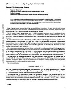
which is further compressed to ad(Z )W = Z 00XS (Z 0). (Readers unfamiliar with this notation for comultiplication are refered to [13].) By taking duals we get the adjoint action of H on B : if Z; X 2 H , and  2 B then ad(Z )()X = (Z 00XS (Z 0)): An element  2 B is invariant if for every Z 2 H , ad(Z ) = (Z ). Our de nition of the adjoint action is chosen so that any function  with the property that (ZW ) = (WZ ) will be invariant. The invariant elements of B form a subalgebra denoted B H . 1.2. A graph consists of a set E called edges, a xed point free involution ? : E ! E , and a partition V of E into subsets called vertices. Let i : E ! V be the map sending e to the vertex v containing it. Let t = i  ?. We call t(e) the terminal vertex of e and i(e) the initial vertex. An orientation is a choice O of one edge from each orbit of the involution. An oriented graph is denoted by the data (E; ?; V; O). There is a one-dimensional CW-complex associated to (E; ?; V; O), which is called its geometric realization. The 0-cells are in one to one correspondence with V , the 1-cells are in one to one correspondence with O, and the characteristic maps are determined by t and i. A ciliation C of a graph is a linear ordering of each vertex. The additional data is denoted V c, although we will continue to use V for the partition of E . A lattice is an oriented, ciliated graph. The geometric realization of an oriented graph is insucient to support a ciliation so for a lattice we construct an oriented surface called its envelope. Each vertex becomes an oriented disk and each edge in O becomes an oriented band. The orientation of a fattened vertex induces an orientation on its boundary, one point of which is marked with a cilium. Attach the band corresponding to each e to the disks (or disk) at its initial and terminal ends. The attaching points along the oriented boundary of each disk must be arranged in the order given by the ciliation of the vertex. Further annotate the resulting surface by orienting the core of each band from i(e) to t(e). For example, consider E = fe1 ; e2 ; e3 ; e4 ; e5 ; e6 ; g; V c = ff?e1 ; e2 g; f?e2; e3g; f?e3 ; e1; e4 ; ?e6g; f?e5 ; ?e4 g; fe6; e5gg and O = fe1 ; e2; e3 ; e4; e5; e6 g;

6

DOUG BULLOCK, CHARLES FROHMAN, AND JOANNA KANIA-BARTOSZYN SKA

Figure 1. Envelope of an oriented, ciliated graph.

Ciliation is given by the order in which the elements of each vertex are written above. The envelope of (E; ?; V c; O) is shown in Figure 1, alongsinde a streamlined schematic version. An envelope determines its lattice. The edge set consists of a pair e for each band, with e assigned to the orientation. Label the initial and terminal ends of a band core by e and ?e respectively. Each disk forms a ciliated vertex by reading o these labels, beginning at the cilium and traveling along the induced orientation. 1.3. For this subsection we x (E; ?; V c; O). A gauge eld theory on this lattice is de ned by the interactions of three algebraic objects: O  A set of connections, A = H .

 A gauge algebra, G =

O e2O v2V

H.

 And a set of gauge elds, C [A ] =

O e2O

B.

The gauge algebra is a Hopf algebra in the natural sense of a tensor power of Hopf algebras, whereas A and C [A ] inherit only the vector space structure of H . However, we will shortly endow the connections with a G -action and a comultiplication, which induce dual structures on C [A ] via the evaluation pairing. For each v 2 V c there is a function ordv : v ! N that assigns to e 2 v the ordinal number corresponding to its position in the ciliation. Connections become a left G -module under the action  (ord (e))  e (e)) : x S y (e) e

v2V yv
e2O xe = e2O y(ord e (e) This is a busy formula, even with the jV j-th order summation over Sweedler notation suppressed. For a graphical description of the action (and the usual method of computing it) see [8]. The gauge algebra acts adjointly on gauge elds via (y
f )(x) = f (y
x), so C [A ] is a right G -module. A gauge eld f is called an observable if for all y 2 G we have y
f = (y)f . Observables form a submodule O of C [A ]. t( )

i( )

i

t

1.4. There is a construction of gauge elds which uses a direct interpretation of the restricted dual of H . Suppose that W is a nite dimensional left H -module. We use W  to denote the dual with H acting on the left by (x
f )(v) = f (S (x)
v). The action (f
x)(v) = f (x
v) makes the dual into a right H -module, denoted

SKEIN MODULES AND LATTICE GAUGE FIELD THEORY

7

W 0. Compultiplication supplies a left action on W  W , namely x
(f v) = (x0
f ) (x00
v). Forcing the natural identi cation of W  W with Hom(W; W ) to be an intertwiner makes the later into a left module as well. In Sweedler notation the action is (y
f )(v) = y00
f (S (y0)
v). Now suppose that  : H ! Hom(W; W ) is the original representation. I.e., x
v = (x)(v). The reader may check that for any x; y 2 H , we have y
(x) = (ad(y)x). A nite dimensional representation  : H ! Hom(V; V ) is said to be adapted to B if fh   j h 2 (Hom(V; V ))0g  B: A coloring of a lattice is a labeling of each e 2 O by a representation adapted to  B . Let We denote the representation associated N to e, and let W?e = We . A coloring naturally associates the left H -module Wv = e2v We to each vertex. Given a coloring, there is a map of right G -modules, O 0 O O Wv ! (W?e We)0 ! (Hom(We; We))0 ! C [A ] v2V

e2O

e2O

de ned as follows. The rst stage is just reordering of the factors with the natural distribution of primes over tensor products. The next is the canonical identi cation. The last is composition with e2O e, where the maps e : H ! Hom(Ve; Ve) are the actual representations of the coloring. Theorem 1. The images of these maps, taken over all colorings, add up to C [A ]. Proof. This is evident after establishing the following claim: For each f 2 B there is a nite dimensional H -module W so that f 2 fh   j h 2 (Hom(W; W ))0g  B: Fix a nonzero f 2 B . Choose I to be maximal among ideals of H contained in ker f . Let  : H ! Hom(W; W ) be the representation induced by left multipication of H on W = H=I . De ne T to be the linear span of the functionals fy 7! f (xyz) j x; z 2 H g. Since I is an ideal and it lies in the kernel of f , T may be thought of as a subspace of W . Choose fx1; : : : ; xng  H so that x1 = 1H and so that, in the quotient, this is a basis for W . By P evaluation, each xi is a functional on T . Suppose that, as a functional on T , X = ai xi = 0. For any y; z 2 H we have f (yXz) = 0. Maximality of I then implies linear independence of fxig on T , which means T is all of W . Choose a basis ff1; : : : ; fng for Wf that is dual to fxig. let (xj ) be the matrix M j in the basis fxig. By duality of bases, we know that every element y 2 H can be written as X y = z + fi(y)xi

where z 2 I . Hence

(y) =

X

fi(y)M i:

8

DOUG BULLOCK, CHARLES FROHMAN, AND JOANNA KANIA-BARTOSZYN SKA

The j -k entry of the matrix (y) is which proves the assertion

X i

fi(y)Mjki ;

fh   j h 2 (Hom(W; W ))0g  B:

Finally, let hj be the function

y 7!

X i

fi(y)Mji1:

Note that hj (xi ) = Mji1. The rst column of M i expresses xix1 in the chosen basis. However, x1 = 1H , so we have Mji1 = ji. Since hj (I ) = 0, we have shown that it agrees with fj on all of H . This proves that fh   j h 2 (Hom(W; W ))0g contains a spanning set for T . In particular, it contains f . If H is semisimple there is a way of getting an isomorphism out of the construction above. Restrict the colors to lie in an exhaustive list of irreducible representations adapted to B , so that no representation appears twice in the list. Once this has been done then the map in theorem above becomes an isomorphism. This is the de nition of gauge elds used in [1, 4]. Let Inv(W ) denote the invariant part of an H -module. Since the maps described above are all intertwiners, we have the following characterization of observables. Corollary 1. The sum over all colorings of the images of Nv2V Inv(Wv ) is equal to O. 2. Multitangles The goal of this subsection is to develop a functor between two categories: the category of multitangles, M, and the category of connections, A. The objects of M are lattices, and a morphism is a set of equivalence classes of tangles in oneto-one correspondence with the vertices of its domain. An object in A is the set of connections on a lattice, viewed as a left module over the gauge algebra of the lattice. The morphisms are pairs of maps, one from the connections in its domain to the connections in its range and the other between the gauge algebras. The second morphism allows us to pull back the connections on the range lattice to a module over the domain gauge algebra. The rst map must intertwine this action with the standard one. A multitangle is described by a collection of diagrams in one-to-one correspondence with the vertices of the domain lattice. Each diagram lies in a copy of [0; 1]  [0; 1] with the second factor determining a height function on the entire collection. Each such collection is built by stacking the elementary diagrams described below. A multitangle is an equivalence class of these collections under a relation that will be made explicit shortly.

SKEIN MODULES AND LATTICE GAUGE FIELD THEORY

9

Figure 2. Identity multitangle.

Figure 3. Negative crossing.

2.1. These are the elementary diagrams.

The identity: The domain and range are the same lattice. For each vertex v

there is a diagram consisting of arcs with no crossings which are monotonic with respect to the height function. The arcs correspond, from left to right, to the cilial ordering of v. Arcs corresponding to edges in the orientation are directed downwards, others are directed upwards. Figure 2 shows an envelope and its identity morphism. The convention for ordering and directing arcs used here is standard for all elementary diagrams. It can also be derived from the envelope of a lattice. Allow the band cores to protrude into a fat vertex and unroll it with a Mobius transformation to the upper half plane, cilium at in nity. Crossings: The domain and range lattices dier only in the ciliation at a single vertex, v, where a pair of adjacent edges have been transposed. At each vertex other than v there is a trivial diagram as in the identity. The diagram at v has monotonic arcs and a single crossing between those arcs corresponding to the transposed edges. Either strand may pass over the other. A geometric example is given in Figure 3. Triads: Consider an involutary pair of edges, e and ?e, in the domain lattice with e 2 O. In the range lattice, e is removed from its position in a ciliated vertex and replaced with e0 ; e00 in that order. Similarly, ?e is replaced with ?e00; ?e0 . The edges e0 and e00 lie in the orientation of the new lattice, which is otherwise identical to the domain. The diagrams have monotonic arcs without crossings corresponding to all the unchanged edges. The two arcs corresponding to e and ?e split at the same

10

DOUG BULLOCK, CHARLES FROHMAN, AND JOANNA KANIA-BARTOSZYN SKA

Figure 4. Triad.

Figure 5. Cap joining a non-involutary pair of edges.

Figure 6. Cup creating an involutary pair at a single vertex.

height into four arcs corresponding to e0, e00 , ?e00 and ?e0 . In an envelop, this is the operation of doubling an edge (Figure 4). Caps: The edge set of the range will dier from the domain by deleting two adjacent edges from a vertex, exactly one of which lies in the orientation. If the two edges are not an involutary pair, then the two orphaned edges in the range become an involutary pair. The strands corresponding to the deleted edges meet at a local maximum. Otherwise the diagrams are trivial. The eect on envelopes is suggested in Figure 5. Cups: The range lattice diers from the domain by introducing two new edges, e and ?e next to each other at a single vertex. The strands corresponding to the new edges originate in a local minimum and obey the usual directedness rule. Otherwise the diagrams are trivial. This creates a monogon at a vertex as shown in Figure 6. Stumps: The range lattice is formed from the domain lattice by deleting an involutary pair of edges. The diagrams are trivial except for the two strands

SKEIN MODULES AND LATTICE GAUGE FIELD THEORY

11

Figure 7. Stump eliminating an involutary pair.

Figure 8. Switch exchanging an involutary pair.

Figure 9. Cut splitting a vertex in two.

corresponding to the deleted edges, which simply terminate. Both stumps must occur at the same height. Figure 7 is an example. Switches: The range diers from the domain by replacing some e with ?e in the orientation. This is indicated in the diagrams by a hash mark on each of the strands involved, with both marks lying at exactly the same height (Figure 8). Cuts: The range lattice is altered by dividing the ordered edges at some vertex into two non-empty consecutive sets, which form new ciliated vertices. The diagram for that vertex is trivial, except for a vertical mark at the top which indicates the cilium of the new vertex (Figure 9). When the range lattice of one collection of diagrams matches the domain of another one may form a new set of diagrams by stacking the two rst two. It may be necessary to isotop the bases to get arcs to match, and if two diagrams are stacked atop a single diagram with a cut, the cut extends to the top of the new diagram. The height function is then uniformly rescaled. We de ne a multidiagram to be any such collection formed by stacking elementary diagrams.

12

DOUG BULLOCK, CHARLES FROHMAN, AND JOANNA KANIA-BARTOSZYN SKA

Figure 10. Generalized Reidemeister moves.

A multidiagram is a picture of a framed embedding of a 1-dimensional CW-complex into a collection of cubes. The 1-cells of this complex are called the segments of the multidiagram. Alternatively, segments are the components left behind if the triads are removed and the arcs passing under a crossing are thought of as connected. A coloring of a multidiagram is an assignment of an irreducible, nite dimensional, H -module to each segment. The critical points, switches, stumps and triads of a multidiagram are collectively refered to as events. 2.2. We say that two colored multidiagrams are equivalent if one can be obtained from the other by a sequence of the following moves.

Isotopies: We allow ambient isotopy of the diagrams subject to the following restricition: No two events sharing a segment may occur at the same height. A pair of marks indicating a stump, switch or triad must always remain at the same height. Cuts must remain vertical. Triads must maintain one segment below the horizontal and two above it. And the events depicted in Figure 12 may not occur at the same height if a pair of involutary edegs is represented among their segments. Generalized Reidemeister Moves: These are shown in Figure 10. The moves are valid regardless of the orientations of the arcs. We also allow the corresponding moves with reversed crossings. Interacting Events: These moves describe the interaction of events that share either a common segment or two segments representing an involutary pair of edges. They are divided into triad moves (Figure 11), cap moves (Figure 12), stump moves (Figure 13) and switch moves (Figure 14). In each picture adjacent pairs of arcs, reading left to right along the base, represent involutary pairs of edges. Subject to that, any orientation of arcs is allowed, as are diagrams with all crossings reversed. The involutary pairs are shown as adjacent merely to conserve space; the moves a valid even for distant arcs. Some of these moves alter the segments. When a segment is created it may appear with any color; a segment that splits in two takes its color to both of the new ones; and in order for two segments to join they must carry the same color.

SKEIN MODULES AND LATTICE GAUGE FIELD THEORY

13

Figure 11. Triad moves.

Figure 12. Cap moves.

Figure 13. Stump moves.

Figure 14. Switch moves.

Algebraic Moves: The two moves in Figure 15 represent fundamental identities

in H : the de nition of S , and R
=
opR. As above, adjacent strands are involutary pairs and colorings must be consistent. De nition 1. A multitangle is an equivalence class of colored multidiagrams.

There is a useful (although somewhat imprecise) topological way of understanding the equivalence of multidiagrams. Think of a multidiagram as a diagram of framed tangles in cubes. For the most part any isotopy relative to the boundary of the cubes is an equivalence, exceptions being the rigidities listed above. Since these involve involutary pairs, and since caps can alter the involution, it is best to be careful when isotoping an event past a cap. Stumps are free to move almost anywhere and they are absorbed (or created) by cups and triads. A switch is a pair of marks that can slide up or down together unless obstructed by a cup, cap or triad. Any pair of switches that meets will cancel (and thus can be created), and a single switch can be canceled (or created) at a cup. A switch can

14

DOUG BULLOCK, CHARLES FROHMAN, AND JOANNA KANIA-BARTOSZYN SKA

Figure 15. Algebraic moves. ty sx

x y

yS (t) sx

x y

S (s)y tx

yS (s) tx

x y

x y

2

ty xS (s)

x y

yS (t) xS (s)

sxS (t)

txS (s)

x y

x

x

S (s)y xS (t)

yS (s) xS (t)

tyS (s)

S (s)xS (t)

x y

x y

x

x

2

2

Figure 16. Action of R and R?1 at crossings.

move up through a triad provided it splits in two, or two switches can combine by moving down through a triad. Triads, moving in pairs, can pass over each other, and a pair merging with a cup creates a pair of cups. Stumps can be retracted or extended at will, and they are absorbed (or created) by cups and triads. In other words, as long as one avoids caps and keeps triads and stumps upright, any continuous deformation of a multitangle is an equivalence and the behavior of cups, stumps, triads, and switches is fairly intuitive. Fortunately, in practical situations caps almost always reside above all other events in the multitangle. If they must be moved about, one can always rely on the list of cap moves. In many applications the coloring of a multitangle is irrelevant. In those cases when it does matter, one rarely sees the moves that alter segments. 2.3. We begin building a functor from M to A by sending a lattice to its connections and the elementary diagrams to the morphisms described below. The identity: This diagram induces the identity on connections and on the gauge algebra. Crossings: The map on connections is an action of the R-matrix or its inverse. There are 12 cases depending on the sign of the crossing, the directions of the arcs, and the possibility that they are an involutary pair. These are given in Figure 16, which describes the action in the factors corresponding to the crossing arcs. The map extends linearly on connections, using the identity in all other factors. The map on the gauge algebra is the identity. Triads: Suppose that e and ?e are replaced by e0, e00, ?e00 and ?e0 , with e 2 O originally. The map on connections is comultiplication in the factor corresponding to e and the identity elsewhere, with the requirement that the image of the comultiplication take values in the tensor product of the factors corresponding

SKEIN MODULES AND LATTICE GAUGE FIELD THEORY x0

x00

x

x00

15

x0

x

Figure 17. Action of a triad. xy

ykx

trV (x)

trV (xk)

x y

x y

x

x

1

k?1

Figure 18. Operators corresponding to cups and caps.

to e0 and e00 in that order. The distribution of the output, using Sweedler notation with summation suppressed, is illustrated in Figure 17. The diagram acts trivially on G . Caps: There are four cases at a local maximum, depending on orientations and on whether or not the incoming strands represent an involutary pair in the domain lattice. These are listed in Figure 18, where trV denotes the ordinary trace taken in the H -module V coloring that segment. If the lattice loses a vertex then the map on G is  in that factor; otherwise it is the identity. Cups: The action on A is either by the unit of H or by the unit followed by multiplication by k?1, depending on the orientation of the cup. The two cases are shown in Figure 18. The map on gauge algebras is the identity. Stumps: A stump acts as the counit in the corresponding factor of the connections. If the range lattice loses one or more vertices because of this, the map on gauge algebras is counit in those factors. Otherwise it is the identity. Switches: For switches the map on connections is x 7! S (xk) in the factor corresponding to the edge. The map on G is trivial. Cuts: A cut has no eect on connections. It acts trivially on G except in the factor corresponding to the split vertex, where the map is
: Hv ! Hv0 Hv00 . Here v0 denotes the initial subset of v after the cut, and v00 the nal subset. A general multidiagram is a composition of elementary ones, so it is sent to the corresponding composition of maps. Theorem 2. Equivalent multidiagrams from ? to ?0 induce identical maps on connections and gauge algebras. The map on connections intertwines the action of G? on A ? with the one on A ?0 pulled back via the map on gauge algebras. Proof. . To check that equivalent multidiagrams induce the same morphisms one must evaluate both sides of each move under every possible arrangement of orientations and crossings. Number the moves in each of Figures 10{15, reading left do right and down the page. We will outline the identities and manipulations in H that make each move invariant on connections. That both sides induce the same map on gauge algebras is elementary.

16

DOUG BULLOCK, CHARLES FROHMAN, AND JOANNA KANIA-BARTOSZYN SKA

Invariance of generalized Reidemeister moves:

1. This follows from the fact that R and R?1 solve the quantum Yang-Baxter equation. 2. Replacing any appearance of S 2(x) with kxk?1 proves invariance in all cases. 3. This is essentially the identity  1(R) = 1 (R) = 1. For some orientations the fact that (S (x)) = (x) is also needed. 4. With the strand directed upwards the left hand side produces the following morphism, where subscripts indicate successive applications of R and implied summation. x 7!xS 2 (s1)kS (t1 ) =xS (t1 k?1 S (s1)) =xS (t1 t2 S 2(s2 )S (s1)) =xS ()S (t1 t2 S (s1S (s2))) =x Similar computations show that, regardless of orientation, both sides act as multiplication by . If the crossings are reversed the action is by ?1 . 5. This similar to (2). 6. Those cases that are not immediate follow from an application of S 2(x) = kxk?1 . 7. RR?1 = R?1 R = 1. 8. Depending on crossings, use one of the identities
1(R) = s1 s2 t1t2 or 1
(R) = s1s2 t2 t1. 9. Obvious.

Triad moves:

1.
(k?1) = k?1 k?1. 2.
is coassociative.

Cap moves:

1. That S is an anti-algebra morphism suces. 2.
is an algebra morphism. 3.  is an algebra morphism and (k) = 1.

Stump moves:

1.  is the counit for
. 2. (k?1) = 1. 3. From earlier identities,  (R1) = 1

Switch moves: 1. S is an anti-coalgebra map and k is grouplike. 2.   S =  and (k) = 1. 3. This is the claim that x 7! S (xk) is an involution. It follows from S 2(x) = kxk?1 . 4. S (k) = k?1. 5. S S (R) = R.

Algebraic Moves:

1. The de nition of S :   S 1 
=   1 S 
=   . 2. Constrained non-cocommutativity: R
(x) =
op(x)R.

SKEIN MODULES AND LATTICE GAUGE FIELD THEORY

17

Checking that every multitangle is a G -module intertwiner is again a matter of checking each elementary diagram under all orientations and crossings. As above, we will indicate the essential identity or manipulation on which the computation rests. Identity: This is obvious. Crossings: Since
coassociative, the identity R
(x) =
op(x)R extends to any adjacent pair of factors in a power of
. In Sweedler notation, y(1)


sy(i) ty(i+1)


y(n) = y(1)


y(i+1) s y(i) t


y(n): This will prove the intertwining of a gauge transformation by y at a single vertex. Any other gauge transformation can be expressed as sums of products of these. Triads: Coassociativity of
again. The proof is trivial in Sweedler notation. Caps: If the valence of the vertex is one or two, the result follows from the de ning equation for S . If the valence is greater than two, we use an extended version of the formula: y(1)


y(n?2) = y(1)


S (y(i))y(i+1)


y(n) = y(1)


y(i)S (y(i+1))


y(n): Cups: These work for pretty much the same reasons that caps do. Stumps: Follows from the de nition of . Switches: S is an anti-algebra map. Cuts: Coassociativity of
.

Remark: We can think of and as single events called positive and negative twists respectively. It is worth remembering that a positive twist acts on a connection as multiplication by ?1 in that factor. A negative twist acts by . 3. Comultiplication of Connections Fix a lattice ? = (E; ?; V c; O). We de ne a multitangle whose domain is ? by repeating the following construction at each vertex: Apply a triad to each arc. Then move the strands corresponding the the x0 's to the left of the the strands corresponding to the x00's so that the latter segments cross over. Finally, cut the diagrams to separate the x0 's from the x00's. An example is given in Figure 19. The multitangle determines a range lattice denoted ? 2 . Its envelope is two disjoint copies of the envelope of ?, but it is important to distinguish then as the prime and double prime copies. The induced morphism on connections is denoted r : A ? ! A ? : The map on gauge algebras is the standard comultiplication on a tensor power of H . We make the identi cation A ? A ? = A ? , and de ne ? = e2O e : A ? ! b: Theorem 3. The triple (A ; r; ?) is a coalgebra. 2

2

18

DOUG BULLOCK, CHARLES FROHMAN, AND JOANNA KANIA-BARTOSZYN SKA

Figure 19. Multitangle for r.

Figure 20. A suggestion of the coassociativity of r

Proof. Figure 20 depicts diagrams for r 1 r and 1 rr at one possible trivlent vertex. To see that the left side is equivalent to the right, slide the higher triads down to the lower ones and then back up the other segments. This is possible because
is coassociative and because the diagrams separate into three disentangled layers. This phenomenon holds in general, and it is possible to organize this information into an inductive proof that r is coassociative. We leave the details to the reader, with the suggestion that one use a coupon, say n

to denote the diagram for r at a generic n-valent vertex. It is also convenient that =

:n ? i The fact that stumps can be retracted and absorbed into triads gives a simple multitangle proof that (? 1)  r = (1 ? )  r = 1. Thus ? is a counit for r. n

i

The adjoint of r, restricted to observables, is denoted by ?: if f; g 2 O and x 2 A , then (f ? g)(x) = (f g)(r(x)).

SKEIN MODULES AND LATTICE GAUGE FIELD THEORY x

yn

1

19

x(n) yn

x(1) y1

y1

Figure 21. Eect of a push on a connection

Corollary 2. O is an algebra under ?. Proof. The intertwining property of morphisms induced by multitangles insures that ? takes values in O. Linearity and associativity follow from linearity and coassociativity of r. The unit is the observable ? .

4. Computing in O The algebra of observables for a lattice should be independent of orientation and should depent only on the cyclic ordering of the ciliated vertices, not the total ordering. Furthermore, mimicking a classical phenomenon, the value of an observable on a connection should be computable from a suitable connection on the complement of a maximal tree in the graph. In this subsection we will x a lattice, (E; ?; V c; O), and prove that these goals can be met. We will also address the interaction of multitangles with the algebra and coalgebra structures from the previous subsection. 4.1. Given e 2 O, let e denote the map on connections induced by the multitangle which is trivial except for a switch on the strands e. In an envelope of ?, e switches the orientation of the core of the corresponding band. Given v 2 V , let

v = jvj?1 ; and v?1 =

jvj?1 :

Here an integer next to an arc indicates that many parallel copies. The orientations are determined by the orientations of the edges at v, and the rest of the multitangle is trivial. The eect on an envelope of v is to toggle the cilium at v one step counterclockwise, while v?1 toggles it the other way. Given e 2 O, let

e =

n

n

where the coupon is
n?1 and the two strands entering it represent e and ?e. The rest of the multitangle is trivial. The domain and range lattices are identical. The eect of the map on a connection is described N in Figure 21, which also introduces the convention of writing a simple tensor in e2O He by labeling the corresponding cores in an envelope. We call this map a push. In order to avoid belaboring useless notation, we will assume that the domains of successive applications of switches, toggles and pushes are clear, provided the original

20

DOUG BULLOCK, CHARLES FROHMAN, AND JOANNA KANIA-BARTOSZYN SKA

domain was speci ed. We will also suppress the subscripts whenever possible. Any sequence of toggles, switches and pushes de nes a G -module map between connection algebras and thus a operator between observables as well. We say that two connections are gauge equivalent if their dierence lies in the span of fy
x ? (y)x j x 2 A ; y 2 Gg. Observables cannot distinguish gauge equivalent connections. Two morphisms in A (with the same domain and range) are gauge equivalent if the images of every connection are gauge equivalent. The adjoints of a pair of gauge equivalent operators are identical maps on observables. Proposition 1. Let f be any sequence of toggles and switches that begins and ends at the same lattice. The induced operator on connections is gauge equivalent to the identity. Proof. It suces to check the compositions  2,     ,     , and vn , where n is the valence of v. Clearly  is an involution. It follows easily from tangle equivalence that the next two are also the identity map. The multitangle for  n is trival away from v. At that vertex it is represented by n

where the coupon denotes the generator (with positive crossings) of the center of the n-strand braid group. Note that it consists only of crossings and twists. Because such a tangle acts as multiplication in the factors corresponding to each segment, its behavior can be understood by its eect on the connection 1. Noting that 1 is grouplike, we can evaluate this as follows:

 n (1) =

n

=

n

=

n

=
n?1 (?1):

Hence, the eect on an arbitrary connection is gauge action by ?1 at v. The same proof with all crossings reversed shows that v?jvj is gauge action by . 4.2. The standard tools for manipulating connections and observables are toggles, switches, pushes, triads (in succession), cups, caps (involving non-involutary pairs), stumps and cuts. We will need an understanding of how well they interact with the coalgebra and algebra structures. We already have notation for the rst three maps. Let
ne be the map induced by a succession of triads on the edges e and ?e. We extend the notation to include
0 for the identity and
?1 for a stump. A cup oriented from e1 to e2 (necessarily involutive) induces the map ee . A cap oriented from e1 to e2 , a non-involutive pair, induces ee . A cut between e1 and e2 (in that order) induces ee . The notation is deliberately parallel with the de ning maps of H , and when context permits we will suppress sub- and superscripts. Theorem 4. The maps ,
n,  and  are coalgebra morphisms. 2 1

2 1

2 1

SKEIN MODULES AND LATTICE GAUGE FIELD THEORY

21

Figure 22. Triad commuting with r at a valence two vertex.

Proof. A switch slides up through the multitangle for r  sigma, becoming a pair of switches on the appropriate edges. Now apply the algebraic move corresponding to R
=
opR to obtain a tangle for    r. Consider the multitangle for    r. At the vertex where the cap occurs we can expand this as

i

2

j

Since the caps do not involve involutary pairs, there is a cap move that makes this into a tangle for r  . The proof that    r = r   is similar. If the lattice has only two edges, the proof that (

)  r = r 
is just Figure 22. If there are more edges a similar proof works because of the layering phenomenon seen in the proof of Theorem 3. Higher powers of
follow immediately;
0 is trivial; and
?1 comes from retracting stumps into triads. In many applications the output of a multitangle is needed only up to gauge equivalence. There is a particular occurrence which can greatly simplify computations. Let  be the operator induced by a multitangle that is trivial except for i

j

:

The dierence between the range and domain lattices is just that a subset of the edges of some vertex has been split o to form a new one. Although there is no multitangle to express it, the identity map on connections is an operator with the same domain and range as . Proposition 2. With notation as above,  is gauge equivalent to the identity. Proof. Given a connection x, we can express (x) as an action of (1) on x, as in the proof of Proposition 1. In the interest of computing (1), replace the i strands of the tangle with a single strand followed by
i?1 . Tangle equivalence allows the triads to

22

DOUG BULLOCK, CHARLES FROHMAN, AND JOANNA KANIA-BARTOSZYN SKA

slide over the crossing, after which we nd that the action is by
i?1 (sj


s2 s1) in the i strands and by t1 t2


tj in the j strands. Now consider the eect of  on x1


xj y1


yi in the factors corresponding to the non-trivial part of the tangle. The result is ti
x1


tj
xj
i?1(sj


s1 )
(y1


yi); where tk
xk means tk yk or yk S (tk ), depending on orientation of the segment, and similarly for
i?1(sj


s1)
(y1


yi). This is exactly gauge action of 1 (sj


s1) on the connection ti
x1


tj
xj y1


yi; which is gauge equivalent to (sj


s1)ti
x1


tj
xj y1


yi: Since  1(R) = 1, this is indistinguishable from the behavior of the identity map. Theorem 5. Up to gauge equivalence,  ,  and  are coalgebra maps. Proof. Draw the tangle for (v v )  r. By Proposition 2 we can replace the cut with jvj

:

The result is equivalent to the tangle for r v . Commutation of  ?1 derives from its gauge equivalence with some power of  . For ( )  r the tangle at the cut vertex is

:

By Proposition 2, this is gauge equivalent to r  . Since  is composed of triads, caps, a cut and a cup, it too commutes up to gauge equivalence. Corollary 3. The adjoints of  , , ,
n, ,  and  restricted to observables are algebra maps. Since  and  are invertible algebra morphisms, we can now see that O is independent of orientation, up to isomorphism, and that it depends only on the cyclic ordering of edges at vertices. 5. Pushes The goal of this section is to prove that a push is invisible to any observable. Let's begin with a basic fact about invariant tensors. Suppose that U and W are left H modules. As in Subsection 1.4, (U  W )0 is a right module. This can be identi ed with Hom(W; U ) as follows: if  2 U  , w 2 W , then h 2 Hom(W; U ) becomes functional

SKEIN MODULES AND LATTICE GAUGE FIELD THEORY

23

sending  w to (h(w)). This isomorphism is an intertwiner if we use the following action: for z 2 H and h 2 Hom(W; U ), (h
z)(w) = S (z0 )
h(z00
w): Lemma 1. If h is invariant then, for all z 2 H and all w 2 W , h(z
w) = z
h(w). Proof. Let y = S ?1 (z). Using Sweedler notation and invariance of h under the action of y0, we have h(z
w) = h(S (y)
w) = h((y0)S (y00)
w) = (y0)h(S (y00)
w) = S (y0)
h(y00
S (y000)
w) = S (y0)
h((y00)w) = S (y)
h(w) = z
h(w):

Now choose a coloring of the lattice with notation e, We, and Wv as in Subsection 1.4. Suppose that our lattice contains the con guration in Figure 21 and that the vertex on the right is v0 = f?e0 ; e1 ; e2; : : : ; eng (with N each0 ei 2 O). Choose a gauge 0 eld of the form f g, where f 2 Wv and g 2 v6=v Wv , and write the connection depicted in Figure 21 as z x y1


yn. The usual N method of evaluation is to convert the gauge eld and the connection into N 0 tensors in e2E We and e2E We, then tensor them together and contract. (Meaning evaluate the functionals in the We0's on the vectors in corresponding We's.) Since these contractions can take place in any order, we can focus on just those taking place between We and We0 for e 2 v0 . To see the invariance of a push, however, we need to think of these contractions as a composition of morphisms. Let W denote We


Wen and let y = y1


yn. Apply e's so that x 2 Hom(We ; We ) and y 2 Hom(W; W ). We can now view f , and hence x  f  y, as a elements of Hom(W; We ). Using standard identi cations, this becomes a tensor in We We


Wen . The evaulation of the full gauge eld is now completed by contractiong g with  (x  f  y). Lemma 2. With notation as above, if f is invariant then x  f  y = 1  f  (x(1) y1




x(n) yn). 0

0

1

0

0

0

0

1

Proof. Choose w 2 W . Reinterpret (x  f  y)(w) as x 2 H acting on f (y(w)). Then apply Lemma 1.

In light of Corollary 1, we have established the following result: Theorem 6. The adjoint of a push is the identity on observables. Corollary 4. Every sequence of toggles, switches and pushes from one lattice to another induces the same isomorphism on observables. Proof. Since pushes induce the identity, is suces to prove this for just toggles and switches. By Proposition 1, any two sequences of toggles and switches are gauge equivalent.

24

DOUG BULLOCK, CHARLES FROHMAN, AND JOANNA KANIA-BARTOSZYN SKA

We have succeed in proving that O is independent of orientation and that it depends only on cyclic ordering at vertices. Also, pushes and corollary 4 indicate that we can evaluate observables on whatever con guration is most favorable for the application at hand. There is one more task. We want to construct (as nearly as possible) a universal description of observables. 6. Quantum holonomy Fix ? = (E; ?; V c; O), with envelope F . We will be quantizing the notion of holonomy along a loop in the lattice. In the classical world, a loop in ? would be just that, the image of an oriented S 1 with base point. However, in order to quantize, we need the image to be generic and to introduce over- and under-crossings. That is, we need a knot diagram, not just a loop. Also, the base point introduces some technicalities. We will refer to the disks in F representing the elements of V as vertices and the bands as edges. Let  be a proper immersion from a disjoint, nite collection of oriented intervals into F , so that endpoints map to cilia, double points lie in vertices, and the image in each edge consists of arcs parallel to the core. Introduce over- and undercrossings at each interior double point. The resulting object is called a q-tangle. The special case when the domain is a single interval is called a q-path if the endpoints are distinct, and a q-loop if not. 6.1. A q-tangle, , determines an operator, hol , from A to a tensor power of H indexed by the components of . It is de ned as the composition of a pair of multitangles connecting a trio of lattices. The rst lattice is ?; the last is determined by the multitangles; the intermediate one comes from , and it is best de ned in terms of its envelope. Its ciliated vertices are the vertices of F that  meets. There is a band along each arc of  in an edge of F , and the cores are oriented by the orientation of . The multitangle connecting the rst two lattices is formed as follows: Apply
m?1 to each pair e, where m is the number of times meets the corresponding edge of F . The range of this morphism is a lattice identical to the intermediate one, described above, except possibly for orientation. Continue the multitangle by inserting switches whenever the orientations disagree. Coloring is irrelevant. The second multitangle is formed from the oriented tangles created by  in each vertex of F . Given a vertex, apply a Mobius transformation mapping it to the upper half plane with the cilium at in nity. Choose a rectangular region that contains all of the image of  except for disjoint arcs running from the top edge to in nity. Rescale this to a unit square. The coloring of the resulting multitangle can be anything compatible with the rst one. The composition of the two induces the operator O Hc: hol : A ! c a component of 

One may think of envelope of the nal lattice as the image of , with fattened endpoints as vertices and ciliation inherited from F .

SKEIN MODULES AND LATTICE GAUGE FIELD THEORY e4

25

e1

e5

e2 e6

e3

Figure 23. Envelope of ? and a q-loop, . x4

x1

x5

x2 x6

S (x005 k)

S (x005 k)

x004 S (x05 k) x006

t2 x004 S (x05 k) x006 S 2 (s2 )

x3

x04

x1 x2

x06

t1 x04

x3

s1 x1 x2

x06

x3

Figure 24. partial computation of hol (x).

6.2. The notation hol is meant to be read, \holonomy along alpha." To see how it is a quantum analog of holonomy, and to illustrate some computational devices, we will work an example where ? and  are as in Figure 23. N Consider the connection x = ei2O xi. Since there is no prescribed ordering to the factors, we express x by labeling each edge of ? with the corresponding xi . With this notation the evaluation of hol (x) | except for the caps in the multitangle | is shown in gure 24. The top picture is x. The middle one is the result of evaluating triads and switches. The nal stage is obtained by evaluating the crossings of the vertex tangle shown in Figure 25. We have left out evaluation of caps because there is an easier way to do it. Traverse the loop, concatenating the symbols accumulated on each edge, and each time you

26

DOUG BULLOCK, CHARLES FROHMAN, AND JOANNA KANIA-BARTOSZYN SKA

x3 x1 x04 x004 x006

x06

Figure 25. Vertex tangle.

pass through a vertex insert k if the cilium lies to your right. This gives hol(x) = t1x04 kS (x005 k)kx06 kt2 x004 kS (x05 k)kx006 S 2(s2 )ks1x1 x2 x3 : In the classical limit k = 1 and R = 1 1, so hol is actually accumulating holonomy as the loop is traversed. Quantization occurs when self intersections become over- or under-crossings. The rules governing appearances of k were arrived at after lengthly experimentation. Their signi cance is still unknown. When a q-path or q-loop has no crossings it makes sense to refer to it by listing the edges traversed. The involution is used to indicate the loop running against the orientation of an edge. For example, with ? and x as above, we have holfe ;e ;e g(x) = x1 x2 x3 = X and holfe ;?e ;e g (x) = x4 S (x5 k)x6 = Y . Properties of S now simplify our computation to hol = t1 (x4 S (x5)kx6 )0kt2 (x4 S (x5)kx6 )00 ks2s1 (x1x2 x3 ) = t1 X 0kt2 X 00ks2s1 Y 1

4

5

2

3

6

In a classical setting holonomy is inverted if the direction of the path is reversed. In a cocommutative Hopf algebra inversion is replaced by the antipode. In a quantum group, however, S is not an involution. So, we have the following quantum analog of the reversing result for holonomy. Proposition 3. Let  be a q-tangle and  the same network but with the orientation of a component c reversed. The operator hol is hol followed by a switch in the factor indexed by c. Proof. hol is de ned by the composition of two multitangles, T1, consisting of stumps and triads followed by some switches, and T2 formed from the vertex tangles. If a switch is inserted between T1 and T2 on every edge coming from c, the resulting multitangle de nes hol . The new switches pass upwards through T2 , canceling at caps, until only one remains. This will lie on a pair of strands corresponding to the component c in the range of the multitangle T2  T1 .

7. Wilson operators There is an equivalence relation on q-tangles which, like the one on multidiagrams, mimics framed tangle isotopy. A base point free q-tangle is the result of smoothing the cusps at the base points of the loops of a q-tangle. Two base point free q-tangles are equivalent if they dier by a sequence of isotopies of F , Reidemeister moves of type II and III, and the framing equivalence = . If one thinks of a base point free q-tangle as a diagram of a framed tangle in F  I , then this equivalence is ambient isotopy xing the endpoints of the acr components and their framing normals.

SKEIN MODULES AND LATTICE GAUGE FIELD THEORY

27

Figure 26. Slides of a q-loop.

A base point free q-tangle can be expanded into a multitangle in the same manner as a based network. Its evaluation, however, will depend on the coloration. Therefore, we de ne an operator for a base point free q-tangle L if and only if each closed component is colored by an irreducible, nite dimensional H -module. The segments of the multitangle created by those components are colored accordingly; the others receive arbitrary colors. The induced map, denoted WL, takes values in a tensor power of H indexed by the uncolored components. Proposition 4. If L and L0 are equivalent base point free q-tangles with the same coloring, then WL = WL0 . Proof. Cerf theory implies L and L0 are equivalent if, within vertices, they dier by the moves of q-tangle equivalence, and outside vertices they dier by the moves in gure 26. These two moves alter multitangles by the two algebraic moves, and the others alter multitangles by generalized Reidemeister moves.

As is usual in knot theory, we use the L to denote both a base point free q-tangle and its equivalence class. The associated operator WL is called a Wilson operator. In the special cases when L consists of closed components, a single closed component, or a single arc component, the operators are called, respectively, a Wilson link, loop, or line. In computing the output of a Wilson operator, we can use the same shortcut for caps as in 6.2. The starting point on a closed component does not matter because trace is invariant under cyclic permutation. Wilson operators obey a reversing result: if the reversed component is an arc the eect is as in Proposition 3, but if it is a closed component its statement requires more care. Suppose that L and L dier by reversing a closed component c colored by V . Let A L denote the connections where WL and WL take values. De ne a map f : A ! Hc A L as follows: Connect c to a base point to obtain a q-tangle L . If the cilium at which c is based lies to its right, then f is WL followed by right multiplication in the factor indexed by c. If it lies to the left, then f = WL . Finally, de ne functions trc and Sc on Hc A L as trV 1 and S 1 respectively. Proposition 5. With notation as above, WL = trc  f and WL = trc  Sc  f

Remark: This is a bit easier to swallow if the L = c. In that case the Wilson loop is computed by taking the trace of something, and the reversed loop is computed by taking S of the trace of something. Proof. Repeat the proof of Proposition 3 up to the point where all but one of the new switches have been canceled. This time the switch will be on two involutary strands entering a cap colored by V . The multitangles for WL and WL dier by replacing

28

DOUG BULLOCK, CHARLES FROHMAN, AND JOANNA KANIA-BARTOSZYN SKA i

j

j

n

n

i

Figure 27. Tangle diagrams for WL and WL  v .

a cap with a switch followed by a reversed cap. Since the rest of the multitangle induces WL , it is easy to verify the proposition for the two possible orientations of the cap. Since multitangles intertwine gauge transformations, Wilson links colored by adapted representations are necessarily elements of O. Furthermore, a Wilson link is determined by a geometric object associated to an envelope. While toggles and switches have no eect on the underlying q-tangle, the alterations to the lattice will eect the evaluation of the Wilson link. Fortunately the variance is natural. Theorem 7. Suppose that ? and ?0 dier by toggles and switches and that f is the induced map on connections. If WL and WL0 are Wilson links built on the same L in the two envelopes, then WL0  f = WL. Proof. Suppose ? and ?0 dier by a switch . The multitangle for WL0 diers from that of WL by a switch on the same edge. Since the switches cancel, we have WL0   = WL. Assume now that the lattices dier by a counterclockwise toggle,  . That part of the multitangle for WL is represented by the left side of Figure 27, where the solid coupons are the switches and powers of
and the dashed coupon contains all the crossings of the transformed vertex. The portion of the multitangle for WL0   at that vertex is now the right side of the gure. Since these are equivalent diagrams, WL0  = WL.

Corollary 5. Let L be a colored base point free q-tangle with no arc components. The unique isomorphism between O? and O0? identi es the Wilson links over L in each algebra. Observables produced by Wilson links can be graphically multiplied. Suppose that L and L0 are equivalence classes of base point free q-tangles with no arcs. Laying L0 over L and perturbing the result creates a new q-tangle denoted L ? L0 . There are several ways to do this, but all are equivalent q-tangles and the result is independent of the representatives used. Theorem 8. WL ? WL0 = WL?L0 . Proof. let F denote the envelope of the lattice. If wt is a tangent vector along a band core, the right hand side of the edge is determined by a normal vector wn so that fwn; wtg is in the orientation of F . By equivalence of q-links, we may assume that L lies to the right of L0 in every edge of F . At each vertex, the multitangle for WL?L0 begins with an arc for each edge of F , oriented accordingly. Apply a triad to each of these arcs so that it splits into a prime branch and a double prime branch. If L meets

SKEIN MODULES AND LATTICE GAUGE FIELD THEORY

29

a given edge m times, apply
m?1 to the prime branch for that edge. If L0 meets it n times, apply
n?1 to the double prime branch. Now insert the necessary switches to make this the rst half of the multitangle. Next, focus on the second part of the multitangle at a single vertex v of F . The transformed vertex ts onto the rst part of the multitangle so that the arcs of L \ v meet the prime branches and the arcs of L0 \ v meet the double primes. Since L lies under L0 one can drag L \ v to the left and L0 \ v to the right until they are disjoint. Finally, move everything between the initial triad on each arc and L \ v to just beneath L \ v, and similarly for L0 \ v. This can be done for every vertex while preserving the simultaneous levels of triads and switches. Inserting a cut in between L \ v and L0 \ v in each diagram, we have a multitangle that represents (WL WL0 )  r. Let bLF denote the linear space over the set of all framed, oriented, colored links in F  I (completed if b = C [[h]]). This is an algebra under ? which|for every ? whose envelope is homeomorphic to F |is identi ed with a sub-algebra W?  O? . Corollary 4 makes these algebras into a category. The content of Corollary 5 is that bLF behaves someaht like a universal object. One of the aims of the next section is to address how much of O is generated by Wilson links.

Part 2. The Structure of the Algebra of Observables In this part of the paper we investigate the structure of the algebra of observables for various choices of H and B . Suppose rst that G is a connected ane algebraic group. We will show that the ring of G-characters of a free group is the algebra of observables for a theory in which H is the universal enveloping algebra of G and B is its coordinate ring. Next we consider the case when H is a Drinfeld-Jimbo deformation of the universal enveloping algebra. Here the observables become a deformation quantization of the classical character ring. Following Fock and Rosly, [10], we show that the Poisson structure with respect to which we are quantizing is the standard Poisson structure, as in the work of [2, 11]. We consider the extent to which one can generate the ring of observables using Wilson loops. Among the groups (and their quantum analogs) for which this is possible is SL2(C ). We conclude with a demonstration that the observables based on (Uh(sl2 ); q SL2 ) are exactly the Kauman bracket skein algebra of a cylinder over the envelope of the lattice. 8. Classical LGFT 8.1. Let's recap a few facts from [12]. An ane algebraic group G is a group equipped with a nitely generated algebra of \polynomial" functions that separate points| the coordinate ring, denoted B |so that multiplication and inversion are polynomial maps. If G is connected then its coordinate ring is naturally identi ed with a stable subalgebra of its universal enveloping algebra, which we denote by H . G acts on itself by conjugation, which adjointly induces and action of G on B . The most important fact for us is that the xed part of B under this action is exactly the ring B H as de ned in Subsection 1.1.

30

DOUG BULLOCK, CHARLES FROHMAN, AND JOANNA KANIA-BARTOSZYN SKA

Now suppose that  is any nitely presented group. A representation of  into G is a point in G 


 G whose coordinates are the images of the generators. These must satisfy polynomial identities corresponding to the relations of the presentation, so the space of all representations is an ane algebraic set. It has a coordinate ring on which G acts by the adjoint of conjugation in each factor. The xed subring|which is independent of presentation (up to isomorphism)|is called the ane G-characters of . We often shorten this to \characters" or \G-characters" when  or G (or both) are understood from context. The notation is XG(). If  is the fundamental group of a compact manifold M , we write XG(M ) for XG (1(M )). 8.2. Fix a connected ane algebraic group G and a lattice ? = (E; ?; V c; O). Let H be the universal enveloping algebra of G and B its coordinate ring, thought of as lying in H o. In order to see what the observables of this theory look like, we rebuild it using groups instead of algebras. Let the connections be the set of functions A : O ! G. The gauge group is the set of functions g : V ! G, and the gauge elds are the set e2O B . We can view the connections as the Cartesian product of copies of G indexed by O. The gauge elds are just the coordinate ring of the Cartesian product. The action of the gauge group on the connections is given by g  A(e) = g(i(e))A(e)g?1(t(e)); where e 2 O, g is an element of the gauge group, and A is a connection. This induces a right action of the gauge group on the gauge elds by taking adjoints. Let OG denote the gauge elds xed by this action. Theorem 9. Let G, H , B , ? = (E; ?; O; V c) and OG be as above, and let O denote the usual observables. 1. O = OG . 2. OG is the G-characters of 1 of the geometric realization of (E; ?; V; O). Proof. 1. Note that the gauge group and the gauge algebra act on the same set of gauge elds. A gauge eld is invariant under the action of the gauge algebra if and only if it is invariant under elements of the form 1


y


1, where y lies in the Lie algebra of G. The proof that these elds are exactly those xed by the gauge group action is now a simple generalization of [12, Corollary IV.3.2]. 2. If the lattice has one vertex containing all the edges then OG is, by de nition, the G-characters of the fundamental group of the geometric realization. For arbitrary ? consider another lattice ?0 that has a single vertex, and so that the two geometric realizations are homotopic. Choose a maximal tree in the geometric realization of ?. There is an obvious map from the connections on ?0 into those on ? that sends them to the edges of O not appearing in the tree. That this is an isomorphism at the level of observables is an elementary exercise.

SKEIN MODULES AND LATTICE GAUGE FIELD THEORY

31

9. Quantized Characters For this subsection we assume that (H; B ) is de ned over C [[h]], and H is a DrinfeldJimbo quantization of a simple Lie algebra g [13]. In this case, H=hH is the universal enveloping algebra of g. We will denote such H by Uh(g). Suppose that B=hB is the coordinate ring of a connected ane algebraic group G. The equivalence of the representation theory of Uh(g) and U (g) makes it easy to see that O=hO is the observables associated to the theory based on (U (g); B=hB ). We use topological tensor products as in [13], so the gauge elds are topologically free. Since observables form a closed subalgebra, it is also topologically free. Therefore the observables based on (Uh(g); B ) are a deformation quantization of the G-characters of the fundamental group of the geometric realization of ?. The only question that remains unanswered is which Poisson structure on the ring of characters is the tangent vector to this deformation. We can assume that Uh (g) has an R-matrix of the form 1 1 + hr + h2a, where a is some formal power series with coecients in U (g) U (g), and r is a solution of the modi ed classical Yang-Baxter equation. In speci c, r 2 g g. Such solutions were classi ed by Belavin and Drinfeld [14]. The standard presentation of U (g) is in terms of generators Xi; Yi; Hi, where i runs over some index set, and each triple generates a copy of U (sl2 ). The Killing form is an element of g g, but being nondegenerate, you can contract it with respect to itself to give an element of g g. This element can be expressed in the form ai Xi Yi + biHi Hi + ciYi Xi. The element r can be assumed to be of the form r = 2ai Xi Yi + bi Hi Hi: There are two actions of r on B B . You can act on the left, by letting r
(f g)(Z1

Z2 ) = f g(r Z1 Z2), or you can act on the right by letting (f g)
r(Z1 Z2) = f (Z1 Z2 r). The Poisson bracket on G is given by ff; gg = (f g)
r ? r
(f g): In order to write out a formula for the Poisson structure, we need to create a version of r that operates on the gauge elds on a lattice. We also need to distinguish left actions and right actions: if Z acts by right multiplication in the factor corresponding to the edge e, we denote it by Z 0(e); if it acts by multiplication on the left, we denote it by Z (e). Since the formula we derive involves antisymmetrization, we let Z1 ^ Z2 = Z 1 Z2 ? Z 2 Z1 . Now suppose that f and g are gauge elds in the quantum theory. One may compute f  g ? g  f by writing it as f g  r ? g f  r, and expanding the R matrix as a power series in h. The linear term is X 2ai Xi0(e) i Y 0(e) + biHi0(e) Hi0(e) ? 2ai Xi(e) i Y (e) ? bi Hi(e) Hi(e)+ e2O

X v2V

?

X <

2aiXi0() ^ Yi0( ) + biHi0() ^ Hi0( )

32

DOUG BULLOCK, CHARLES FROHMAN, AND JOANNA KANIA-BARTOSZYN SKA

?

X ?