plicable to skeletonize gray-scale images from boundaries di- rectly. We start from ... N} be be all the boundary segments and L(si) is the length of si. We partition S into .... 7. REFERENCES. [1] Nicu D Cornea, Deborah Silver, and Patrick Min.,.
SKELETONIZATION OF GRAY-SCALE IMAGE FROM INCOMPLETE BOUNDARIES Quannan Li, Xiang Bai, WenYu Liu Huazhong University of Science and Technology,Wuhan,P.R.China ABSTRACT Skeletonization of gray-scale images is a challenging problem in computer vision due to the difficulty of segmenting grayscale images to get the complete contour. Compared with previous skeletonization algorithms which use computational methods to avoid segmentation, this paper reveals that it is applicable to skeletonize gray-scale images from boundaries directly. We start from boundaries of gray-scale images and perform Euclidean Distance Transform on boundaries. Then we compute the gradient magnitude of the distance transform and perform isotropic vector diffusion. After diffusion, the Skeleton Strength Map (SSM) is computed and skeleton can be extracted from SSM. The experiments show that this method can obtain good skeleton from boundaries so long as major boundary segments are preserved. Index Terms— Skeletonization, Incomplete Boundary, Skeleton Strength Map, Isotropic Vector Diffusion 1. INTRODUCTION
of narrow objects effectively without losing information. But for objects that are wider, this algorithm fails because heavy blurring is needed for wide objects and many details would be lost. In [4], anisotropic vector diffusion is used to address the bias problem, but this algorithm also fails to extract skeleton of wide objects. In [5], the authors proposed a method that extracts the skeletons from a set of level-set curves of the edge strength map and in [6], an approach is proposed to deal with the situation where the objects are always brighter or darker than the background. In [7], [8], methods are proposed based on scale-space theory and extract the ”cores” from the ridges of a medialness function.In [9], a thinning algorithm is proposed to skeletonize the gray-scale images using a pseudo-distance. These segmentation-free algorithms avoid the step of segmentation, however, as we have mentioned above, we can benefit a lot from a contour. In this paper we illustrate that we can extract good skeleton from boundary segments, even not a connected contour, so long as major boundary segments are preserved. We first perform distance transform on boundary and then perform isotropic vector diffusion on the gradient vector field of the distance transform. After diffusion, we compute the skeleton strength map (SSM). We can either threshold the SSM to get the skeleton or select local maxima with the aid of body map in [10] to obtain the ultimate connected skeleton. To remove insignificant boundary segments, a simple heuristic is used. In the experiment, we shall that, we can extract good skeleton from the boundary obtained by Canny operator or the boundary obtained by algorithms combined with learning in [10].
Skeleton is an important shape descriptor for object representation and recognition since it can preserve both topological and geometrical information. It has important applications in object representation and recognition, such as image retrieval and processing, character recognition, computer graphics and biomedical image analysis. Broadly used skeletonization approaches can be categorized into four types [1]: thinning algorithms, discrete domain algorithms based on the Voronoi diagram, algorithms based on distance transform, and algorithms based on mathematical morphology. The common requirement of the above 2. SKELETONIZATION FROM INCOMPLETE algorithms is that the contour of a shape is needed before its BOUNDARIES skeletonization. There are two advantages in skeletonization when we get a complete shape contour: 1) we can use con2.1. Noise Smoothing tour to determine the inner-side and out-side of one object; 2) Since skeleton is a local quantity, it is easily influenced by we can quantify the global significance of skeleton branches noises. Therefore we should remove noisy boundaries before based on the contour [2] skeletonization. Here we propose a simple criterion to delete However, due to the difficulty of image segmentation, these algorithms fail to work on gray-scale images. Many segmentation-insignificant boundary segments, where boundary segments denote paths between any two endpoints that have only one free skeletonization algorithms are then proposed. In [3], a neighbor. novel computational algorithm is proposed to compute a We use two heuristics to quantify the significance of edge segpseudo-distance map directly from the original image using ments: 1) longer boundary segments are more significant than a nonlinear governing equation. It can compute the skeleton
short boundary segments and 2) if one short boundary segment is next to a long segment,it is still possible to compute skeleton branches from them, so we shall treat one short segment more significant if its endpoints are nearer to endpoints of a long segment. To implement these two heuristics,suppose S = {si |1 ≤ i ≤ N } be be all the boundary segments and L(si ) is the length of si . We partition S into two subsets S1 = {s,i |1 ≤ i ≤ N1 } and S2 = {s,,i |1 ≤ i ≤ N1 } (N1 + N2 = N )containing segments longer or shorter than a threshold T1 respectively. For each boundary segment s,,i in S2 , we compute the distance of its endpoints to all endpoints of segments in S1 . If the minimum distance is greater than certain threshold, we treat this segment as noise and remove it.This process can be illustrated by Fig 1. Fig.1 (b) shows the boundary of Fig.1 (a) obtained by canny operator, and Fig.1 (c) shows the boundaries after removing insignificant segments. We can see that, removing some short segments with endpoints distant from endpoints of long segments don’t affect the whole shape of the horse.
Fig. 1. Illustration of the effect of eliminating insignificant edge segments. (b) the boundary of (a) and (c) the boundary with insignificant segments deleted.
2.2. Skeleton Strength Map (SSM) In SSM the value at each point indicates the probability of this point being a skeleton point. The advantage of SSM has been discussed in [11]: it has large value in pixels where skeleton points should be and the values decreases faster to zero when the distance from the skeleton increases. This is a very good property since we can easily decide the skeleton from SSM. Unlike [11] which deals with binary images only, here we extend it into gray-scale images. To compute the SSM, the boundary is firstly reversed and the Euclidean distance transform is performed. We reverse the edge map because in grayscale images, we cannot decide whether one pixel is inside or outside the object since we don’t have the contour. In such case, we treat all pixels except pixels at boundaries as pixels of the object. We apply isotropic diffusion to diffuse the gradient of the distance transform. This diffusion process is ruled by a partial differential equation set as in [12], {
du dt du dt
= µ∇2 u − (u − fx )(fx2 + fy2 ) = µ∇2 v − (u − fy )(fx2 + fy2 )
(1)
Here,µ is the regular parameter,u,v are two components of the diffused gradient vector field,f (~r) = 1 − k∇Gσ (~r) ∗
Fig. 2. Illustration of computation of SSM. (a) the distance transform; (b) shows the SSM (c) the SSM thinned by nonmaxima suppression; (d) the SSM after SSM value assigned 0 at boundaries; (e) the skeleton and (f) the skeleton put back onto the original image.
dt(~r)kwhere Gσ (~r) is the Gaussian kernel function,σ is its standard covariance and ∗ is the convolution operator.fx and fy are the two components of f (~r). Initializing u,v with ∂f (u0 , v0 ) = ∇f = ( ∂f ∂x , ∂y ), the partial differential equation (1) can be solved iteratively by finite difference technique. We use isotropic diffusion because it makes the vectors propagate towards the actual location of the skeleton points. This is very important in order to get the accurate skeleton. Moreover, it is an efficient way of smoothing noise, which makes the extracted skeleton robust to boundary noise. We denote by gvf (~r) the diffused gradient vector field obtained by (2) at point ~r and them SSM (~r) can be computed by formula(2)
SSM (~r) = max(0,
X ~ r , ∈N (~ r)
)
gvf (~r) · (~r − ~r, ) k~r − ~r, k
(2)
Where N (~r) denotes the eight-neighbors of ~r. We then use non-maxima suppression to thin the regions in which SSM is non-zero to one pixel wide. The process is similar as the suppression in Canny operator. We can see its effectiveness from Fig.2 (c) that the SSM has been thinned by non-maxima suppression. As we can see from Fig.2 (c), there are still high values on SSM caused by boundaries. It is easy to remove them since we have known the boundary in advance. Constructing for each boundary pixel a window of size k ∗ k and assigning SSM values at pixels within that window 0 (k = 3 will generally suffice) will remove such values. Fig. 2 (d) shows the SSM after high values caused by boundaries removed. Using hysteresis thresholding, we can get the ultimate skeleton (Fig.2 (e, f) show the skeleton and the skeleton put back onto the original image).
3. SKELETONIZATION FROM BOUNDARIES IN [10] Boundaries obtained from canny operator are insufficient for us to decide the region of object since it captures only low-level information. If we can combine some high-level information, we can compute better skeleton. [10] proposes a algorithm called auto − context that learns an integrated low-level and context model and can get good boundaries and body map that indicates the probability a pixel belonging to the object (Fig. 3(a, c) shows respectively the boundary and body map obtained by the algorithm in [10].). We illustrate that our method has the potential to get good skeleton from boundaries and body map by [10]. We also delete insignificant boundary segments to remove noises in order to get clearer boundary (Fig.3 (b)) and compute the SSM from boundary as depicted in section 2.2 (Shown in Fig.3 (e)). Instead of thresholding SSM, we can skeletonize the grayscale further since we have body map now and can use body map to decide the inner-side and out-side of the object. For each pixel p, we use the average probability of its neighborhood to quantify its probability inside the object. We construct a circle with radius r and compute the average probability of p0 s neighbor within this circle. (Shown in Fig.3 (d), r = 6). By multiplying the SSM with the probability computed, we can now reduce the SSM values at pixels outside the object (shown in Fig. 3(f)). We then select the local maxima from SSM and use Di-
Fig. 3. Illustration of Skeletonization from boundaries computed by [10]. (a) the boundary from [10]; (b) the boundary with noise removed; (c) the body map from [10]; (d) the blurred body map; (e) the SSM; (f) the SSM after reducing values outside the object; (g) local maxima; (h) the skeleton on the original image (the segments in red). jkstra’s shortest distance algorithm to connect local maximum pixels to form the ultimate skeleton. This process is very similar to [11]. The gradient path is defined as the path with minimum sum of magnitude of gradient and corresponds to a geodesic path on the surface defined by
Fig. 4. (a) original images; (b) the edge by canny operator;(c) the SSM; (d) the skeleton; (e) results by [4] f (~r) = 1 − k∇Gσ (~r) ∗ dt(~r)k. We obtain the skeleton by connecting the local maximum pixels with the gradient paths. Fig.3. (h) shows the result of connecting all the local maximum pixels of Fig.4.(g). Note that, since we use shortest distance algorithm, the skeleton branches computed are of one pixel width. 4. EXPERIMENTS In this section we present some results and comparisions. T1 can be set between 20 and 30pixels in our experiments. Fig.4. shows two skeletonization results from boundaries of Canny operator. We can see that although there are lots of gaps, e.g. gaps on back of the dog, and gaps on feet of the horse, we still we can compute quite good skeleton strength maps (shown in column (c)). Column (d) shows the skeleton (in red) obtained by thresholding the skeleton strength map. Although the skeleton is not connected due to thresholding, for each major part of the object, there are skeleton branches corresponding to those parts, e.g. the head and legs of the dog. Column (e) shows the comparison results of the two examples (the skeleton is shown in yellow) obtained by the segmentation-free method proposed by [4]. Compared with [4], our results have one obvious advantage: the skeleton is much more symmetric to the boundary of the objects. This can be seen from the torsos of the dog and the horse. The red lines are much more centered than the yellow lines. In addition, our results have completer skeleton on the legs. These advantages benefits from the usage of the cleaning boundary.
Fig. 5. Comparison of this method with algorithm proposed in [13]; (a) the original image; (b) the SSM; (c) the skeleton obtained from SSM; (d) the skeleton obtained by algorithm in [13].
[2] X. Bai, L.J. Latecki, and W.-Y. Liu, “Skeleton pruning by contour partitioning with discrete curve evolution,” IEEE Trans. Pattern Anal.Mach. Intell, vol. 29, pp. 18– 23, 2007. [3] J.H. Jang and K.S. Hong, “A pseudo-distance map for the segmentation-free skeletonization of gray-scale images,” Proc. Intl Conf. Computer Vision, vol. 2, pp. 18– 23, 1920. Fig. 6. Some results of skeletonization from boundaries [10]. (a) the boundaries from [10]; (b) the body maps; (c) the SSM; (d) the local maxima; (e) the final skeleton;
[4] Zeyun Yu and Chandrajit Bajaj, “A segmentation-free approach for skeletonization of gray-scale images via anisotropic vector diffusion,” Proc.Computer Vision and Pattern Recognition, pp. 18–23, 2004.
In Fig. 5, we compare our method with the algorithm incorporating curvature effect into current damping proposed in [13] (Fig.5 (d)). We can see that although the skeleton obtained by the proposed method is computed from boundary directly, it is comparable to Fig.5 (d) in completeness of the skeleton. In addition, the branches of the skeleton by our method are much more clean and clear. Fig.6. illustrates that with the aid of body map, we can obtain good skeleton from boundaries. Though there are a lot of noises and gaps among the boundaries, clear SSM be obtained (Fig.6(c)) and good skeleton can be extracted (Fig. 6(e)).
[5] S. Tari, J. Shah, and H. Pien, “Extraction of shape skeletons from gray-scale images,” Computer Vision and Image Understanding, vol. 66, pp. 133–146, 1997.
5. CONCLUSION Considering skeleton is easily affected by local noises, we propose a novel method to extract skeleton from significant boundaries. We apply isotropic vector diffusion and compute SSM from the original boundaries. We can either thresholding the SSM to get the skeleton or select local maxima with the aid of body map to form the ultimate connected skeleton. We have also proposed a simple criterion to delete insignificant boundary segments. The experiments show that our method can achieve quite good performance. Our future work include how to extract robust skeletons of gray-scale images with boundary completion. 6. ACKNOWLEDGEMENT
[6] D.H. Chung and G. Sapiro, “Segmentation-free skeletonization of gray-scale images via pdes,” Intl Conf. Image Processing, vol. 62, pp. 927–930, 2000. [7] S.M. Pizer, D. Eberly, D.S. Fritsch, and B.S.Morse, “Zoominvariantvision of figural shape: The mathematics of cores,” Computer Vision and Image Understanding, vol. 69, pp. 55–71, 1998. [8] B.S. Morse, S.M. Pizer, D.T. Puff, and C. Gu, “Zoominvariant vision of figural shape: Effects on cores of images disturbances,” Computer Vision and Image Understanding, vol. 69, pp. 72–86, 1998. [9] A. Nedzved, S. Ablameyko, and S. Uchida, “Gray-scale thinning by using a pseudo-distance map,” Proc. Intl Conf. Pattern Recognition, vol. 2, pp. 239–242, 2006. [10] Zhuowen Tu, “Auto-context and its application for highlevel vision,” Accepted by CVPR2008. [11] Longin Jan Latecki, Quan-nan Li, Xiang Bai, and Wenyu Liu, “Skeletonization using ssm of the distance transform,” Proc. Intl Conf. Image Processing, vol. 5, pp. 349–352, September 2007. [12] C. Xu and J.L. Prince, “Snakes, shapes, and gradient vector flow,” IEEE Trans. Image Processing, vol. 7, pp. 359–369, 1998.
This work was supported by a grant from the Ph.D. Programs Foundation of Ministry of Education of China (No.20070487028 [13] Huaijun Qiu and Edwin R. Hancock, “Gray scale im). We would like to thank Dr.Tu Zhuowen in UCLA for proage skeletonisation from noise-damped vector potenviding us with the data set of body map. tial,” Proc. Intl Conf. Pattern Recognition, vol. 2, pp. 839–842, August 2004. 7. REFERENCES [1] Nicu D Cornea, Deborah Silver, and Patrick Min., “Curve-skeleton properties, applications, and algorithms,” IEEE Visualization, vol. 29, pp. 449–462, 2007.