Sketch-Based Image Retrieval By Size-Adaptive and Noise-Robust Feature Description Houssem Chatbri∗ , Keisuke Kameyama† , and Paul Kwan‡ ∗ Graudate
School of Systems and Information Engineering, Department of Computer Science, University of Tsukuba, Japan † Faculty of Engineering, Information and Systems, University of Tsukuba, Japan ‡ School of Science and Technology, University of New England, Armidale, NSW 2351, Australia ∗
[email protected] †
[email protected] ‡
[email protected]
Abstract—We review available methods for Sketch-Based Image Retrieval (SBIR) and we discuss their limitations. Then, we present two SBIR algorithms: The first algorithm extracts shape features by using support regions calculated for each sketch point, and the second algorithm adapts the Shape Context descriptor [1] to make it scale invariant and enhances its performance in presence of noise. Both algorithms share the property of calculating the feature extraction window according to the sketch size. Experiments and comparative evaluation with state-of-theart methods show that the proposed algorithms are competitive in distinctiveness capability and robust against noise.
I.
I NTRODUCTION
Since the appearance of web search engines in the early nineties, the common way to search for images was by providing text keywords that explain what is the image about. Then, the search engine brings the images which annotations include some of or all the words introduced by the user [2]. In the early years of image searching, this paradigm of image search was convenient enough. However, the explosive growth of storage capacities made manual image annotation a very tedious task [3], and hence encouraged research on alternatives for image retrieval using text keywords. Such alternatives should describe images by other means than text annotations. For a start, that will remove the dependence of the annotation to a particular language. In addition, it is largely argued that text-based annotation is limited, subjective and biased [4]: Two people will describe a same image, very likely, by two different descriptions and that will depend on their cultural backgrounds, their affiliations, and even their emotional states. The automatic image description technique that is sought should be objective and should come from the image content itself and not from the person describing it. Early efforts in this research field, called Content-Based Image Retrieval (CBIR), go back to Kato et al. with their system called Query by Visual Example (QVE) [5] and IBM’s Query by Image and Video Content (QBIC) system [6]. In both systems, the user submits an ”example image” which was collected or hand-drawn, and the system retrieves the database images which look visually similar to the user query. This paradigm is automatic, does not require text annotations of the database images, and will not depend on a particular language or cultural background, which makes it objective. CBIR has been applied in many application domains such as image copyright checking where a user can check if his/her image has been used illegally [7], medical imaging where a
doctor can find similar cases to help the diagnosis process by finding medical images similar to the one he/she holds [8], law enforcement where police detectives can find photos of suspects by submitting to a CBIR system the sketch photo that an expert drew using the information given by a witness [9], etc. A typical CBIR system works as follows: the user will submit a query image, and the system will extract features, or descriptors, that describes the visual content of the query image. Then, these features are matched against a feature database, that has been generated by applying feature extraction on an image database. Finally, the images which features match the query features are output to the user. A particular doctrine in CBIR is the one that is concerned with the use of sketch images as queries to retrieve sketch or full color images. A sketch query is usually a black and white hand-drawn image, which is the main characteristic behind the particularity of this doctrine. The particularity lies in the difference between sketches and full color images in the image content representation. While in full color images, the color information can be used as features, in sketch images only the shape information is available [10]. This area of research is referred to as Sketch-Based Image Retrieval (SBIR). The SBIR paradigm offers to users the possibility of expressing their thoughts with a drawing, which is of particular interest when the query cannot be expressed by text keywords, nor an example image is available. However, dealing with hand-drawn sketches adds in the challenge of user drawing style variance [11], in addition to the issue of noise that exist usually in sketch images [12]. Many SBIR algorithms have been introduced and their performance has been evaluated in several applications. While they have been proven efficient, most methods are still vulnerable in presence of noise. In this work, we review available SBIR methods and we discuss their limitations. Then, we present two SBIR algorithms: The first algorithm extracts shape features by using support regions calculated for each sketch point, and the second algorithm adapts the Shape Context descriptor [1] to make it scale invariant and enhances its performance in presence of noise. Both algorithms share the property of calculating the feature extraction window according to the sketch size. Hence, they differ to existing methods in the feature extraction mechanism that is size-adaptive and tuned to deal with noisy data. Experiments and comparative evaluation with
state-of-the-art methods show that the proposed algorithms are competitive in distinctiveness capability and robust against noise.
Graph-based methods represent a sketch image using a graph-like structure, and matching is done by using graph matching methods.
The outline of this manuscript is as follows: in Sec. II, we review available SBIR methods. In Sec. III and Sec. IV, we explain the two SBIR algorithms in details. Experimental results and comparative evaluation are discussed in Sec. V. Sec. VI concludes the work.
Statistical approaches are less sensitive to noise than graphbased methods, while graph-based methods pave the way for allowing partial matching [23].
II.
R ELATEDW ORK
We start by explaining our classification methodology. Then, we review SBIR methods and we discuss their limitations. A. Classification methodology Online and offline methods: Sketch images can be introduced online [11][13], using a sketch input device (e.g. a tablet), or offline [11][14] by scanning images or using computer graphics. In case where the query is introduced on-line, the time information, namely the order in which sketch points have been introduced, is available and can be used as additional information [10][15][11]. Within this paradigm, a sketch is considered as a set of strokes (line segments), each defined as the set of points (consisting of geometrical coordinates and time) sampled between pen down and pen up events [13]. When the sketch is introduced offline, the time information is not preserved and the sketch is dealt with as a bitmap [11]. Online methods that rely on the time information suppose that the sketch database has been introduced online as well, hence they are not adequate image retrieval on a database introduced offline. Global and local methods: Methods for sketch-based image retrieval can be classified as global and local methods. Global methods [16][17] generate features based on the coarse information of the sketch image, and hence do not carry much information about the local details surrounding a sketch point. As for local methods, they generate features using the point local neighborhood, therefore they are more capable of capturing fine details of the sketch. Global features are robust against noise [18], yet not very distinctive. On the other hand, local features are able to provide more distinctiveness, since they capture fine details. However, they are less robust against noise [18]. This has motivated approaches combining global and local information in order to achieve good distinctiveness and keep fair robustness against noise [1][19]. Statistical and Graph-based methods: Another classification for sketch-based image retrieval is into methods that use a statistical feature representation [17][1][19][20] and methods that use a graph-based feature representation [21][22]. In statistical approaches, sketch images are represented by feature vectors using methods from the rich statistical repository such as shape pixel distributions [17][1][19] and shape signatures [18], and matching is done using a distance or a similarity function.
B. State-of-the-art review Many methods have been proposed for sketch-based image retrieval. In this section, we review important methods and label them using the classification described in the previous section. Kato et al. designed a pioneer system on sketch-based image retrieval [5] called Query by Visual Example (QVE). The system takes hand-drawn sketch queries and retrieves similar full color images. The hand-drawn queries are subjected to a preprocessing step consisting of size normalization and thinning, while database images are transformed to edge images before applying the same preprocessing. When a query image and database image are to be matched, they are first decomposed into equal sized blocks, then local correlation of the corresponding blocks, along with global correlation between the two images, are used to generate a similarity score. The QVE method is a statistical method, combining global and local information, and it is based on the assumption that edges are informative since users draw sketches that try to follow the edge of objects they want to retrieve. However, the variations in drawing styles makes it hard to match two rough sketches by use of correlation. Another method that uses the edge information assumption is Angular Partitioning [17]. In this method, an image is first decomposed into K directional slices. Then, sketch points in each slice are counted to form a feature vector {f (0), ..., f (K − 1)} where f (i) is the number of sketch points located within slice i. The authors use the 1-D discrete Fourier transform to introduce rotation invariance. Finally, the image feature vector corresponds to the K frequency components {|F (0)|, ..., |F (K − 1)|}, where F (u) is the 1dimensional Fourier transform. The Manhattan distance is used for similarity measurement. Angular Partitioning is a global statistical method, fast and easy to implement. However, relying only on global features fails to provide high distinctiveness. Kumagai et al. tackle this limitation by combining global and local features. Their method, called Edge Relational Histogram (ERH) [19][24], works as follows: for each sketch point, the local 8 connected pixels are used to extract local features, and the distribution of sketch pixels in 8 directions is used to extract global features. the local features and the global features are stored in 8 components features arrays, then converted into decimal numbers and used to populate a two dimensional histogram that is used as a feature vector. ERH combines global and local features to generate a statistical feature vector. The authors report results of comparative experiments with two global methods and a local method. ERH achieves the best performances, proving that combining local and global features contributes to improving
the distinctiveness of sketch features. In addition, the method is invariant to translation and scale, while rotation and symmetry invariance can be achieved by generating multiple histograms per single image, corresponding to each orientation or symmetry. However, because of the use of pixel-scale local features, the method is sensitive to noise. The Shape Context (SC) [1] method combines local and global features in another way. First, N points are sampled from the sketch image border points using uniform spacing sampling. Then, for each sample point p, all vectors originating from p to the remaining N − 1 sample points are considered to build a 5 × 12 histogram, where 5 and 12 bins represent the vectors’ norms and angles. The 5 × 12 histogram, h(p), is called the Shape Context of p. The sketch is then represented by the set {h(p1 ), ..., h(pn )} containing Shape Contexts of the sampled N points. When two sketches are matched, all Shape Contexts of the first sketch are compared with all Shape Contexts of the second sketch using a distance function, then the similarity between the two sketches is expressed by the cumulative minimum distance of all histograms comparison. SC is a statistical method that combines local and global features. During the point sampling step, SC performs a uniform spacing sampling and does not privilege interest points such as corners, crossing points or endpoints. Due to the point by point matching scheme, SC is robust against noise yet considerably time-consuming [25]. Moreover, the SC method needs a sketch points sampling policy, which has been shown in other works [26] to be a critical parameter to set, and that it is highly dependent to the size of the sketch [27]. In addition, the size of the feature extraction window is static and not adaptive to the scale of the image, which makes SC not scaleinvariant. Unlike Shape Context, the Curvature Scale Space (CSS) method introduced by Mokhtarian et al [28][29], distinguishes between sketch points and represents a sketch by its interest points. The CSS technique studies the evolution of shape S within a Scale Space Filtering [30], and represents S using the curvature zero-crossing points (inflection points) of the shape curvature function, which is called the shape signature. As the blurring factor σ increases, the shape of Sσ changes. The plot of feature points with variant σ is called the CSS image. The shape is finally represented by locations of its CSS contours maxima. The representation is robust with respect to noise, scale and orientation changes, and its application to CBIR showed good distinctiveness [29]. The CSS method is a global statistical method, designed to deal only with closed concave contours; Convex and complex shapes are poorly represented with the technique. In [31], Kopf et al. describe an attempt to extend the CSS technique and make it able to represent convex shapes. Their idea is to create a mapping of the original shape to a second shape, called mapped shape, where strong convex segments of the original shape become concave segments of the mapped shape, and significant curvatures in the original shape remain significant in the mapped shape. The mapping is done by enclosing the sketch with a circle of radius R and locate the point P of the circle closest to each sketch pixel. The sketch pixels are then mirrored on the tangent of the circle in P . The center of the circle is the average position of sketch pixels.
Other approaches using shape signatures have been introduced. In [32], Zhang and Lu compares the performances of 4 shape signatures when used to calculate Fourier descriptors. The shape signatures are complex coordinates, centroid distance, cumulative angular function, and curvature function. Results show that the centroid signature is the best among the 4 shape signatures, and performances of the complex coordinates and cumulative angular function are comparable, while the performance of the curvature function is poor. Other methods tried to represent sketches by their strokes. In [33], Leung and Chen presented a method for matching hand-drawn sketches based on geometrical features. A preprocessing step is first performed to resample the sketch into a fixed number of points, then strokes which endpoints are close are merged. Each stroke forming the sketch is represented by a 3-dimensional feature vector that expresses the stroke likelihood to 3 types of shapes: line, circle and polygon. Sketches are then compared stroke-by-stroke. The authors applied their feature representation in a sketch-based trademark retrieval in [34]. The database images used in [34] are binary trademark images, and the query is a hand-drawn sketch. The authors applied a preprocessing step on the database consisting of noise reduction, then a segmentation of the image into separated regions according to pixel connectivity, and finally sketch extraction by edge detection or thinning. Deciding to perform edge detection or thinning is carried dynamically for each image region based on studying the distribution of the distance between skeleton pixels and their nearest contour pixels. The approach using dynamic sketch extraction gave the best result, followed by results of using static sketch extraction by edge detection, and finally by thinning. Leung and Chen’s method [33] is a statistical method that generate features using the structure of the sketch. The method can be described as local since features are generated for each stroke of the sketch. For this purpose, a segmentation step is needed to decompose a sketch into its strokes. The segmentation step is crucial for following sketch processing, and due to the fact that there is no formal definition for segmentation points of freehand sketches, it is difficult to evaluate a sketch segmentation result [35][36]. Namboodiri and Jain also used stroke-based feature representation in [16]. Their method works as follows: First, the sketch points are resampled to form a sketch less affected by the noise coming from digitization and pen vibration. The resampling takes equidistant points from each stroke forming the sketch, then connects these points forming smooth lines. Then, each stroke forming the sketch is decomposed into stroke segments in locus where either the x or y coordinate changes its direction. Finally, each stroke segment is represented by a 3-dimensional feature vector including the stroke segment’ position, direction and length. Sketch matching is performed by computing a weighted Euclidean distance. Namboodiri and Jain’s method [16] is an online global statistical method, that requires point sampling and segmentation. The point sampling policy, which is equidistant sampling in this case, has been proven to be crucial step difficult to configure [26] and dependent to the size of the sketch [27]. In addition, the segmentation step is also crucial and can be ambiguous [35][36].
Other approaches represent a sketch using the relations between its strokes. In [21], Leung and Chen introduced a method called Hierarchical Matching that represents a sketch by a hierarchical tree. First, sketch strokes are merged using the same method as in [33]. Then, the parent-child hierarchy is examined between every pair of strokes and used to build a hierarchical tree. The authors define the parent-child hierarchy as the child stroke being contained inside the parent stroke using bounding boxes. In addition to the hierarchical tree, each stroke is represented by 3 features: •
Hyper-stroke features, which represents a parent stroke with all its descendent strokes using Hu moments [37] and the histogram of edge orientations [38].
•
Stroke features, which are geometrical features that express the likelihood of the stroke to fall into a class of geometrical shapes (e.g. line, circle, polygon, etc.).
•
Bistroke features, which expresses the spatial relation between strokes in the same hierarchical level.
During the matching stage, two sketches are first compared in a top to bottom hierarchical manner using their stroke features, and the number of similar strokes is considered as a first similarity measure. Then, a second similarity measure is computed by counting how many corresponding stroke pairs preserve also the parent-child hierarchy. Hierarchical Matching is a graph-based method, which makes it capable of partial matching. However, it has been shown to be sensitive to noise [23]. C. Summary Sketch-based image retrieval methods can be classified according to whether they are implemented online or offline, according to the type of features they use: whether global or local, or also according to their feature representation paradigm: whether statistical or graph-based. Online implementations provides the stroke order information that can be used as an additional feature, in which case database images should be introduced online as well. Offline methods do not require the time information to be present, which make them less restrictive compared to online methods. Global methods are robust against noise, yet they fail to provide high distinctiveness. On the other hand, local methods provide more distinctiveness, at the expense of robustness against noise. A natural tendency was to combine local and global features hoping to achieve a good tradeoff between distinctiveness and robustness against noise. Graph-based methods offer the possibility of performing partial matching, however, their most important limitation is their weakness against noise.
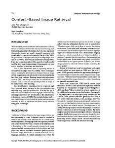
sketch points is first calculated as follows (Fig. 1(a) and Fig. 1(b)): N 1 X dmean = distance(p, pi ) (1) N i=1 where N is the total number of sketch points, pi is a sketch →: point and distance(p, pi ) returns the norm of the vector − pp i − → distance(p , p) = kpp k (2) i
i
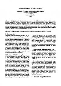
Second, from the perspective of p, sketch points are classified into near region pixels and far region pixels, as follows: IF distance(p, ps ) ≤ dmean THEN ps ∈ Near Region ELSE ps ∈ Far Region where ps is a sketch point. Sketch points located in each region are counted within 8 directions (Fig. 1(c) and Fig. 1(d)) to generate two 8-component features, fc(near) and fc(f ar) , relative to each region (Fig. 1(e) and Fig. 1(f)). Afterwards, a normalization is performed by dividing each 8-component feature by the sum of all bins of that feature, generating fn(near) and fn(f ar) (Fig. 1(g) and Fig. 1(h)). Then, a thresholding is performed to generate binary valued 8-component features, fb(near) and fb(f ar) (Fig. 1(i) and Fig. 1(j)): IF fn [k] < θ THEN fb [k] ← 0 ELSE fb [k] ← 1 where θ is the binarization threshold chosen empirically and k is the bin index of the 8-component feature. Next, the two binary 8-component features are used to generate two binary numbers, bnear and bf ar , by concatenating bins’ entries from a starting bin in an anti-clockwise direction (Fig. 1(i) and Fig. 1(j)). Finally, the two binary numbers are converted into decimal numbers dnear and df ar . The couple (dnear , df ar ) is used to populate a 256 × 256 feature histogram H. The feature histogram H is normalized by dividing by the sum of all bins. Fig. 2 illustrates SRD’s robustness against noise. Although the sketch image in Fig. 2(b) contains a significant amount of noise comparing to the sketch image in Fig. 2(a), the correspondence between their respective histograms is 61%. The similarity measure, defined in Sec. III-B, in this case was equal to 0.70. ERH [24], which uses a histogram-based feature representation, delivers 10% of correspondence and a similarity measure equal to 0.24. B. Matching When a sketch query and a database sketch are to be matched, their corresponding feature histograms, H q and H db , are compared using the Histogram Intersection similarity measure [39], S, defined as follows:
S=
255 X 255 X
q db min(Hgl , Hgl )
(3)
g=0 l=0
III.
SBIR A LGORITHM 1
A. Feature extraction The first SBIR algorithm, which we call Support Regions Descriptor (SRD), works as follows (Fig. 1): For each sketch point p the average distance, dmean , from p to all the other
S takes real values in the interval [0, 1]. When two sketches are similar, S takes values near 1. Otherwise, S takes small values near 0. Because the near and far support regions are defined adaptively for each sketch point by calculating dmean , the
Bin 3
Bin 2
Bin 1
p Bin 4
Bin 5
(a) Input skeleton image and point p 4
12
4
8
0
2
0
0
0 0
8
(e) fc(near)
(b) Sketch segmented using dmean corresponding to p 0
13
9
0.14
0
0
0
0
(f) fc(f ar)
0.42
0.28
Bin 6
Bin 7
(c) Feature extraction layout
0.14
0.25
0
0.06
0
0
(g) fn(near)
Bin 0
0
0.28
1
0
0
0
0
0.4
(h) fn(f ar)
(d) Feature extraction layout as seen from p 1
1
1
1
0
0
0
0
(i) fth(near)
0
1 0
1
0
(j) fth(f ar)
Fig. 1. Feature extraction process: (a) Input skeleton image and an arbitrary sketch point p. (b) Near region (green) and far region (blue) highlighted for point p. (c) Feature extraction layout. (c) Feature extraction layout as seen from p. (e) Near region’s sketch points count. (f) Far region’s sketch points count. (g) Near region’s feature after normalization. (h) Far region’s feature after normalization. (i) Near region’s feature after thresholding. The feature generates the binary number (01000100)2 . (j) Far region’s feature after thresholding. The feature generates the binary number (01001010)2 .
A. Feature extraction
(b)
0
Global features
Far regions features
255
255
(a)
SISC works as follows: For each point p ∈ {p0 , ..pN −1 }, where N is the number of sketch points, the average distance, dmean , from p to all the other sketch points is first calculated as follows: N 1 X −→ dmean = kppi k (4) N − 1 i=1
Near regions features
255
0
Local features
(c)
255
(d)
Next, the feature extraction window is adjusted to be of a r = 2 × dmean radius. All vectors originating from p to sketch points located within the feature extraction window are considered to build a n×m histogram, where n and m bins are used to represent the vectors’ norms and angles. n and m are chosen empirically. The norm bins have equal sizes and each norm bin samples points located in the interval [k nr , (k + 1) nr ] where k is the bin index and takes values in {0, .., n − 1}. The n × m histogram is called the Scale-Invariant Shape Context (SISC) of p.
Fig. 2. SRD’s robustness against noise: (a) Neat sketch. (b) Noisy Sketch. (c)(d) Overlapped feature histograms of SRD and ERH corresponding to images in (a) and (b). The blue dots show overlapping non-zero bins, while the red dots are non-zero bins existing only in the histogram of the noisy sketch.
Calculating the feature extraction window’s size in a dynamic manner according to the distribution of sketch points relative to each point p insures scale-invariance. Fig. 3 shows an example of how the window adjusts its size accordingly to the sketch scale.
approach is invariant to scale. Rotation invariance can also be introduced by generating multiple feature histograms for the query per rotation shift.
B. Matching
IV.
SBIR A LGORITHM 2
The second SBIR algorithm introduces a feature extraction mechanism similar to Shape Context (SC) [1], but with using a dynamic feature extraction window that is size-adaptive. Hence, we call it Scale-Invariant Shape Context (SISC).
When two sketches are matched, all SISC of the first sketch are compared with all SISC of the second sketch using the X 2 statistic. Let p and q be two points of sketches S1 and S2 . The X 2 statistics of histograms g and h corresponding to p and q is calculated as follows: Cp,q =
K−1 1 X [g(k) − h(k)]2 2 g(k) + h(k) k=0
(5)
Sn,1
r
(a)
Sn1,0 Sn,0
(a)
Sn,m
Fig. 4.
(b)
(c)
Examples from the sketch image database.
(b)
Fig. 3. Feature extraction layout in SISC: (a) A small sketch. (b) A large sketch. The feature extraction window is size-adaptive.
(a) Fig. 5.
(b)
(c)
Examples from Dataset 1 generated using [40].
where Cp,q is the X 2 statistic between two SISC histograms g and h, K = n × m is the number of histogram bins, and k is the bin index. The distance, d, between the two sketches S1 and S2 is calculated as the cumulative minimum distance of all histograms, as follows: NX 1 −1 (6) d= min {Ci,j } i=0
(a) Fig. 6.
(b)
(c)
Examples from Dataset 2 generated using ATF [12].
0≤j