Sep 8, 2014 - space streaming algorithm for a (1 â ε)-approximation of Max-Cut follows ..... We generalize Karger's min-cut algorithm to hypergraphs, and then show that its ..... Random sampling in cut, flow, and network design problems.
Sketching Cuts in Graphs and Hypergraphs Dmitry Kogan∗ Robert Krauthgamer∗ Weizmann Institute of Science
arXiv:1409.2391v1 [cs.DS] 8 Sep 2014
September 9, 2014
Abstract Sketching and streaming algorithms are in the forefront of current research directions for cut problems in graphs. In the streaming model, we show that (1 − ε)-approximation for MaxCut must use n1−O(ε) space; moreover, beating 4/5-approximation requires polynomial space. For the sketching model, we show that r-uniform hypergraphs admit a (1 + ε)-cut-sparsifier (i.e., a weighted subhypergraph that approximately preserves all the cuts) with O(ε−2 n(r + log n)) edges. We also make first steps towards sketching general CSPs (Constraint Satisfaction Problems).
1
Introduction
The emergence of massive datasets has turned many algorithms impractical, because the standard assumption of having (fast) random access to the input is no longer valid. One example is when data is too large to fit in the main memory (or even on disk) of one machine; another is when the input can be accessed only as a stream, e.g., because its creation rate is so high, that it cannot even be stored in full for further processing. Luckily, the nature of the problems has evolved too, and we may often settle on approximate, rather than exact, solutions. These situations have led to the rise of new computational paradigms. In the streaming model (aka data-stream), the input can be accessed only as a stream (i.e., a single pass of sequential access), and the algorithm’s space complexity (storage requirement) must be small relative to the stream size. In the sketching model, the input is summarized (compressed) into a so-called sketch, which is short and suffices for further processing without access to the original input. The two models are related – sketches are often useful in the design of streaming algorithms, and vice versa. In particular, lower bounds for sketch-size often imply lower bounds on the space complexity of streaming algorithms. Graph problems. Recently, the streaming model has seen many exciting developments on graph problems, where an input graph G = (V, E) is represented by a stream of edges. The algorithm reads the stream and should then report a solution to a predetermined problem on G, such as graph connectivity or maximum matching; see e.g. the surveys [Zha10, McG14]. Throughout it will be convenient to denote n = |V |, and to assume edges have weights, given by w : E → R+ . While ∗
Work supported in part by a US-Israel BSF grant #2010418, Israel Science Foundation grant #897/13, and by the Citi Foundation. Email: {dmitry.kogan,robert.krauthgamer}@weizmann.ac.il
1
initial efforts focused on polylogarithmic-space algorithms, various intractability results have shifted the attention to what is called the semi-streaming model, where the algorithm’s space complexity 1 In general, this storage is not sufficient to record the entire edge-set. ˜ is O(n). Cuts in graphs is a classical topic that has been studied extensively for more than half a century, and the last two decades have seen a surge of attention turning to the question of their succinct representation. The pioneering work of Bencz´ ur and Karger [BK96] introduced the notion of cut sparsifiers: given an undirected graph G = (V, E, w), a (1 + ε)-sparsifier is a (sparse) weighted subgraph G0 = (V, E 0 , w0 ) that preserves the value of every cut up to a multiplicative factor 1 + ε. Formally, this is written as ¯ w0 (S, S) ∀S ⊂ V, 1≤ ≤ 1 + ε; ¯ w(S, S) 1 , which affects ε ≤ 12 but it is sometimes convenient to replace the lefthand-side with 1 − ε or 1+ε by only a constant factor. In addition to their role in saving storage, sparsifiers are important because they can speed-up graph algorithms whose running time depends on the number of edges. Observe that sparsifiers are a particularly strong form of graph-sketches since on top of retaining the value of all cuts, they hold the additional property of being subgraphs, rather than arbitrary data structures. 2 )-space ˜ Ahn and Guha [AG09] built upon the machinery of cut sparsifiers to present an O(n/ε streaming algorithm that can produce a (1 + ε)-approximation to all cuts in a graph. Further improvements handle also edge deletions [AGM12a, AGM12b, GKP12], or the stronger notion of spectral sparsification (see [KLM+ 11] and references therein). These results are nearly optimal, due to a space lower bound of Ω(n/ε2 ) for sketching all cuts in a graph [AKW14] (which improves an earlier bound of [AG09]).
Recent Directions. These advances on sketching and streaming of graph cuts inspired new questions. One direction is to seek space-efficient streaming algorithms for specific cut problems, such as approximating Max-Cut, rather than all cuts. A second direction concerns hypergraphs, asking whether cut sparsification, sketching and streaming can be generalized to hypergraphs. Finally, viewing cuts in graphs and hypergraphs as special cases of constraint satisfaction problems (CSPs), we ask whether other CSPs also admit sketches. Currently, there is a growing interest in generalizing graph cut problems to broader settings, such as sparsifying general set systems using small weighted samples [NR13], high-dimensional expander theory [KKL14], sparsest-cuts in hypergraphs [LM14, Lou14], and applications of hypergraph cuts in networking [YOTI14].
1.1
Our Results
We first address a natural question raised in [IMNO11, Question 10], whether the well-known Max-Cut problem admits approximation strictly better than factor 1/2 by streaming algorithms that use space sublinear in n. Here, Max-Cut denotes the problem of computing the value of a maximum cut in the input graph G (and not the cut itself), since reporting a cut requires space Ω(n) (see Subsection 2.2 for a short proof). We prove that for every fixed ε ∈ (0, 15 ), streaming algorithms achieving (1 − ε)-approximation for Max-Cut must use n1−O(ε) space. In fact, even beating 4/5-approximation requires polynomial space. Our result is actually stronger and holds also in a certain sketching model. Previously, it was known that streaming computation 1
˜ ) to denote O(f polylog f ), which suppresses logarithmic terms. We use O(f
2
of Max-Cut exactly requires Ω(n2 ) bits [Zel11]. Our proof is by reduction from the Boolean Hidden Hypermatching problem, and captures the difficulty of distinguishing, under limited communication, whether the graph is avertex-disjoint union of even-length cycles (in which case the graph is bipartite) or of odd-length cycles (in which case we can bound the maximum cut value). See Section 2 for details. Second, we study sparsification of cuts in hypergraphs, and prove that every r-uniform hyper2 ) that approximates all cuts ˜ graph admits a sparsifier (weighted subhypergraph) of size O(rn/ε within factor 1 ± ε. This result immediately implies sketching and streaming algorithms (follow¯ in a hypergraph H = (V, E, w) is the total weight of ing [AG09]). Here, the weight of cut (S, S) ¯ 2 This question was raised by de Carli Silva all hyperedges e ∈ E that intersect both S and S. et al. [dCHS11, Corollary 8], who show that every r-uniform hypergraph has a sparsifier of size O(n) that approximates all cuts within factor Θ(r2 ). As hypergraph cuts can be viewed as setsystems, sparsifiers of size O(n2 ), regardless of r, follow implicitly from [NR13]. Along the way, we establish interesting, if not surprising, bounds on the number of approximately minimum cuts in hypergraphs. Technically, this is our most substantial contribution, see Section 3 for details. Finally, as a step towards understanding a wider range of CSPs, we show that k-SAT instances 2 ) that can be used to (1 + ε)-approximate the value ˜ on n variables admit a sketch of size O(kn/ε of all truth assignments. We prove this result in Section 3.3 by reducing it to hypergraph sparsification. We remark that sketching of SAT formulae was studied in a different setting, where some computational-complexity assumptions were used in [DvM10] to preclude a significant sizereduction that preserves the satisfiability of the formula. Our sparsification result differs in that it approximately preserves the value of all assignments. Related Work. Independently of our work, Kapralov, Khanna and Sudan [KKS14] studied the same problem of approximating Max-Cut in the streaming model. They first prove that for every fixed ε > 0, streaming algorithms achieving (1 − ε)-approximation for Max-Cut must use n1−O(ε) space. (This is similar to our Theorem 2.1.) They then make significant further progress, and show ˜ √n) space. that achieving an approximation ratio strictly better than (the trivial) 1/2 require Ω( In fact, this result holds even if the edges of the graph are presented in a random (rather than adversarial) order.
2
Sketching Max-Cut
The classical Max-Cut problem is perhaps the simplest Max-CSP problem. Therefore, it has been studied extensively, leading to fundamental results both in approximation algorithms [GW95] and in hardness of approximation [KKMO04]. It is thus natural to study Max-Cut also in the streaming model. As mentioned above, preserving the values of all cuts in a graph requires linear space even if only approximate values are required [AG09, AKW14], which raises the question whether smaller space suffices to approximate only the Max-Cut value (as mentioned above, it is natural to require the algorithm to report only the value of the cut as opposed to the cut itself, see Section 2.2). P ¯ The latter definition seems Another possible definition, see [dCHS11, Corollary 7], is e∈E we · |e ∩ S| · |e ∩ S|. technically easier for sparsification, although both generalize the case of ordinary graphs (r = 2). 2
3
� ˜ n2 Sketching all cuts in a graph clearly preserves also the maximum-cut value, and thus an O ε space streaming algorithm for a (1 − ε)-approximation of Max-Cut follows immediately from [AG09]. Yet since the maximum cut value is always Ω(m), where m is the total number (or weight) of all edges, a similar result can be obtained more easily by uniform sampling (achieving εm additive approximation for all cuts) [Zel09, Theorem 21]. The latter approach has the additional advantage that it immediately extends to hypergraphs. It turns out that this relatively straightforward approach is not far from optimal, as we prove that streaming algorithms that give a (1 − ε)-approximation for Max-Cut require n1−O(ε) space. Theorem 2.1. Fix a constant ε ∈ (0, 15 ). Every (randomized) streaming algorithm that gives a (1 − ε)-approximation of the Max-Cut value in n-vertex graphs requires space Ω(n1−1/t ) for 1 t = b 2ε − 12 c, which in particular means space n1−O(ε) . To prove this result, we consider the somewhat stronger one-way two-party communication model, where instead of arriving as a stream, the set of edges of a graph is split between two parties, who engage in a communication protocol to compute (approximately) the graph’s maximum-cut value. Since a lower bound in this model immediately translates to the original streaming model, the theorem above follows immediately from Theorem 2.3 below.
2.1
Proof of Theorem 2.1
Definition 2.2 (Max-Cutε ). Let G = (V, EA ∪ EB ) be an input graph on |V | = n vertices with maximum cut value3 c∗ , and ε > 0 some small constant. Max-Cutε is a two player communication game where Alice and Bob receive the edges EA and EB respectively and need to output a value c0 such that with high probability (1 − ε)c∗ ≤ c0 ≤ c∗ . Theorem 2.3. Fix a constant ε ∈ (0, 15 ). Then the randomized one-way communication complexity 1 of Max-Cutε is Ω(n1−1/t ) for t = b 2ε − 12 c. The proof is by a reduction from the following communication problem studied in [YV11]. Definition 2.4 (BHHtn ). The Boolean Hidden Hypermatching problem is a communication complexity problem where • Alice gets a boolean vector x ∈ {0, 1}n where n = 2kt for some integer k, • Bob gets a perfect hypermatching M on n vertices where each edge has t vertices and a boolean vector w of length n/t. L L Let M x denote the length-n/t boolean vector ( 1≤i≤t xM1,i , . . . , 1≤i≤t xMn/t,i ) where (M1,1 , . . . , M1,t ) , . . . ,(Mn/t,1 , . . . , Mn/t,t ) are the edges of M. It is promised that either M x ⊕ w = 1n/t or M x ⊕ w = 0n/t . The problem is to return 1 in the former case, and to return 0 in the latter. Lemma 2.5 ([YV11, Theorem 2.1]). The randomized one-way communication complexity of BHHtn where n = 2kt for some integer k ≥ 1 is Ω(n1−1/t ). 3
For the proof of the lower bound it suffices to restrict our attention to unweighted graphs, with all edges having unit weight.
4
Proof of Theorem 2.3. We show a reduction from BHHtn to Max-Cutε . Consider an instance (x, M, w) of the BHHtn problem: Alice gets x ∈ {0, 1}n , and Bob gets a perfect hypermatching M and a vector w ∈ {0, 1}n/t . We construct a graph G for the Max-Cutε problem as follows (see Figure 2.1 for an example): 2n/t
2n • The vertices of G are V = {vi }2n i=1 ∪ {ui }i=1 ∪ {wi }i=1 .
• The edges EA given to Alice are: for every i ∈ [n], if xi = 0, Alice is given two “parallel” edges (u2i−1 , v2i−1 ), (u2i , v2i ); if xi = 1, Alice is given two “cross” edges (u2i−1 , v2i ), (u2i , v2i−1 ). • The edges EB given to Bob are: for each hyperedge Mj = (i1 , i2 , . . . , it ) ∈ M (where the order is fixed arbitrarily): – For k = 1, 2, . . . , t − 1, Bob is given (u2ik −1 , v2ik+1 −1 ) and (u2ik , v2ik+1 ) – For k = t, Bob is given (u2it , w2j ) and (v2it −1 , w2j−1 ); – If wj = 0 Bob is given two “parallel” edges (w2j , v2i1 ) and (w2j−1 , v2i1 −1 ); if wj = 1, Bob is given two “cross” edges (w2j , v2i1 −1 ) and (w2j−1 , v2i1 ) Pt By definition, for each j ∈ [n/t], if Mj = (i1 , i2 , . . . , it ) ∈ M and (M x)j ⊕ wj = 0 we have k=1 xik ⊕ wj = 0. Since the number of 1 bits in the latter sum is even, when we start traversing from u2i1 we go through an even number of “cross” edges and complete a cycle of length 2t + 1. Similarly when starting our traversal at u2i1 −1 we complete a different cycle of the same length. Therefore if (x, M, w) is a 0-instance the graph consists of 2n t paths of (odd) length 2t + 1 each. 2n ∗ Therefore the maximum cut value is c0 = 2t · t = 4n. On the other hand if (M x)j ⊕ wj = 1, starting our traversal at u2i1 −1 , we pass an odd number of cross edges and end up at u2i1 , from where we once again pass an odd number of cross edges, to complete a cycle of total length 2 · (2t + 1) = 4t + 2 that ends back in u2i1 −1 . Therefore, if (x, M, w) is a 1-instance the graph consists of n/t paths of (even) length 4t + 2 each. The maximum cut value in this case is c∗1 = 4n + 2 nt . 4n 2t Observing that c∗0 /c∗1 = 4n+2n/t = 2t+1 < 1 − ε, we conclude that a randomized one-way ε 0 protocol for Max-Cut (on input size n = 4n + n/t = O(n)) gives a randomized one-way protocol for BHHtn . By Lemma 2.5 the Theorem follows. Proof of Theorem 2.3. Any streaming algorithm for Max-Cutε leads to a one-way communication protocol in the two party setting. Moreover the communication complexity of this protocol is exactly the space complexity of the streaming algorithm. Hence by Theorem 2.3 the streaming space complexity is at least as high as the one way randomized communication complexity.
2.2
Reporting a Vertex-Bipartition (rather than a value)
We show a simple Ω(n) space lower bound for reporting a vertex-bipartition that gives an approximate maximum cut. Proposition 2.6. Let ε ∈ (0, 21 ) be some small constant. Suppose sk is a sketching algorithm that outputs at most s = s(n, ε) bits, and est is an estimation algorithm, such that together, for every nvertex graph G, (with high probability) they output a vertex-bipartition that gives an approximately ¯ ≥ (1 − ε)w maximum cut; i.e., est(sk(G)) = S such that w(S, S) ˜ where w ˜ is the maximum cut in G. Then s ≥ Ωε (n). 5
v1
v2
v3
v4
v5
v6 w1
u1
u2
u3
u4
u5
w2
u6
Figure 1: An example of a gadget constructed in the proof of Theorem 2.3 for t = 3, a matching M that contains the hyperedge M1 = (1, 2, 3), x1 = 1, x2 = 0, x3 = 1 and w1 = 0. The result is two paths of length 7. Alice’s and Bob’s edges are colored black and red respectively. %vspace20pt
Proof. Let C ⊂ {0, 1}n be a binary error-correcting code of size |C| = 2Ω(n) with relative distance ε. We may assume w.l.o.g. that for every x ∈ C the hamming weight |x| is exactly n/2 (for instance by taking C 0 = {x¯ x : x ∈ C} where x ¯ denotes the bitwise negation of x), and that there are no x, y ∈ C such that |x − y¯| ≤ 2ε n (since for every x ∈ C there could be at most one “bad” y, and we can discard one codeword out of every such pair). Fix a codeword x ∈ {0, 1}n and consider the complete bipartite graph Gx = (V, E) where V = [n] and E = {(i, j) : xi = 0 ∧ xj = 1}. The maximum cut value in Gx is obviously w ˜ = n2 /4. Let y ∈ {0, 1}n such that 12 εn ≤ |x − y| ≤ n2 . Identifying x, y with subsets Sx , Sy ⊆ [n], and using the fact that |Sx 4Sy | = |x − y| ≥ 21 εn, the value of the cut (Sy , S¯y ) in Gx is �n � �n � n2 n2 |E(Sy , S¯y )| = − |Sx \ Sy | − |Sy \ Sx | − |Sy \ Sx | − |Sx \ Sy | < (1 − Ω(ε)) 4 2 2 4 Let sk(Gx ) be the sketch of Gx , and let est(sk(Gx )) = S be the output of the estimation algorithm on the sketch of Gx . Therefore if the sketch succeeds (which by our assumption happens ¯ has value at least (1 − Ω(ε))w, with high probability) and the cut (S, S) ˜ then by the preceding argument the corresponding vector xS is of relative hamming distance smaller than 2ε from x and then one can decode x from S.4 By standard arguments from information theory, the size s of a sketch that succeeds with high probability must be at least Ω(log |C|) = Ωε (n).
2.3
2/3-Approximation of Max-Cut in the Two Party Model
We remark that in the one-way two-party model, the parameter range ε ∈ (0, 15 ) in Theorem 2.3 is tight and not merely a technical limitation of our analysis. In that model, the problem of 4 ¯ S) has the same value as (S, S), ¯ the vector xS can actually be ε-close to x Since the cuts (S, ¯, but by taking our code to have no codeword being close to the negation of another codeword we can always try decoding both xS and x ¯S .
6
2t -approximation of the maximum cut exhibits an exponential gap in the communication giving a 2t+1 complexity between the case of t ≥ 2, where we have shown that a polynomial number of bits is necessary, and the case t = 1, for which logarithmically many bits suffice, as follows from the following simple protocol.
Proposition 2.7. Let G = (V, EA ∪· EB ) be an input graph on |V | = n vertices. Let wA and wB be the maximum cut values in GA = (V, EA ) and GB = (V, EB ) respectively. Then it holds for the maximum cut value w in G 2 3 (wA + wB ) ≤ w ≤ wA + wB Proof. Consider cuts CA , CB : V → {0, 1} such that w(CA ) = wA and w(CB ) = wB . Let C : V → {0, 1} be a cut chosen uniformly at random from {CA , CB , CA + CB }. For an edge e = (u, v) ∈ CA , either CB (u) + CB (v) = 1 or (CA + CB )(u) + (CA + CB )(u) = (CA (u) + CA (v)) + (CB (u) + CB (v)) = 1 + 0 = 1. Either way PrC∈R {CA ,CB ,CA +CB } [e ∈ C] = 32 . Similarly the same holds for an edge e ∈ CB . Therefore by linearity of expectation a random cut in {CA , CB , CA + CB } has value at least 32 (wA + wB ). The second inequality is trivial. Corollary 2.8. The one-way communication complexity of Max-Cut1/3 is O(log n). Proof. Alice computes the value wA and sends it to Bob. Bob computes the value wB and outputs 2 3 (wA + wB ).
3
Sketching Cuts in Hypergraphs
In a celebrated series of works, Karger [Kar95, Kar98, Kar99] and Bencz´ ur and Karger [BK96, BK02] showed an effective method to sketch the values of all the cuts of an undirected (weighted) graph G = (V, E, w) by constructing a cut-sparsifier, which is a subgraph with different edge weights, that � ˜ n/ε2 edges, and approximates the weight of every cut in G up to a multiplicative contains only O factor of (1 ± ε). We generalize the ideas of Bencz´ ur and Karger to obtain cut-sparsifiers of hypergraphs, as stated below. Such sparsifiers (and sketches) can be computed by streaming ˜ algorithms that use O(rn) space for r-uniform hypergraphs using known techniques (of [AG09] and subsequent work). Theorem 3.1. For every r-uniform5 hypergraph H = (V, E, w) and an error parameter ε ∈ (0, 1), there is a subhypergraph Hε (with different edge weights) such that: � • Hε has O n(r + log n)/ε2 hyperedges. • The weight of every cut in Hε is (1 ± ε) times the weight of the corresponding cut in H. A key combinatorial property exploited in the Bencz´ ur-Karger analysis is an upper bound on the number of cuts of near-minimum weight [Kar93]. It asserts that in the number of minimum-weight cuts in an n-vertex graph is at most n2 (which had been previously shown by [LP72] and [DKL76]), and more generally, there are at most n2α cuts whose weight is at most α ≥ 1 times the minimum. Correctly generalizing this property to r-uniform hypergraphs appears to be a nontrivial question. A fairly simple analysis generalizes the latter bound to nrα , but using new ideas, we manage to obtain the following tighter bound. 5
Throughout this work we allow r-uniform hypergraphs to contain also hyperedges with less than r endpoints (for instance by allowing duplicate vertices in the same hyperedge).
7
Theorem 3.2. Let H = (V, E, w) be a weighted r-uniform hypergraph with n vertices and minimum cut value w. ˆ Then for every half-integer α ≥ 1, the number of cuts in H of weight at most αw ˆ is at most O(2αr n2α ). We prove this “cut-counting” bound in Section 3.1. With this bound at hand, we prove Theorem 3.1 similarly to the original proof of [BK96] for graphs, as outlined in Subsection 3.2. Cuts in hypergraphs are perhaps one of the simplest examples of CSPs, with the hypergraph vertices becoming boolean variables, and the hyperedges becoming constraints defined by the predicate Not-All-Equal. A natural question is whether general CSPs admit sketches as well, where a sketch should provide an approximation to the value of every assignment to the CSP (as usual, the value of an assignment is the number of constraints it satisfies). Although we are still far from answering this question in full generality, we prove that for the well-known SAT problem, sketching is indeed possible. Theorem 3.3. For every error parameter ε ∈ (0, 1), there is a sketching algorithm that produces 2 ), that can be used to (1 ± ε)˜ from an r-CNF formula Φ on n variables a sketch of size O(rn/ε approximate the value of every assignment to Φ.
3.1
Near-Minimum Cuts in Hypergraphs
In this subsection we prove our upper bound on the number of near-minimum cuts (Theorem 3.2). We generalize Karger’s min-cut algorithm to hypergraphs, and then show that its probability to output any individual cut is not small (Theorem 3.4), which immediately yields a bound on the number of distinct cuts. Finally, we show that the exponential dependence on r in Theorem 3.2 is necessary (Section 3.1.3). 3.1.1
A Randomized Contraction Algorithm
Consider the following generalization of Karger’s contraction algorithm [Kar93] to hypergraphs. Algorithm 3.1 ContractHypergraph Input: an r-uniform weighted hypergraph H = (V, E, w) a parameter α > 1 Output: a cut C = (S, V \ S) 1: H 0 ← H 2: while |V (H 0 )| > αr do 3: e ← random hyperedge in H 0 with probability proportional to its weight 4: contract e by merging all its endpoints and removing self-loops6 5: C 0 ← random cut in H 0 (bipartition of V (H 0 )) 6: return the cut C in H induced by the cut C 0 6
Here by self-loops we refer to hyperedges that contain only a single vertex. Note also that the cardinality of an edge can only decrease as a result of contractions.
8
Theorem 3.4. Let H = (V, E, w) be a weighted r-uniform hypergraph with minimum cut value w, ˆ let n = |V |, and let α ≥ 1 be some half-integer. Fix C = (S, V \ S) to be some cut in H of weight Qn,r,α for at most αw. ˆ Then Algorithm 3.1 outputs the cut C with probability at least 2αr−1 −1 Qn,r,α
� � 2α + 1 n − α(r − 2) −1 = (r + 1) 2α
Since Theorem 3.4 gives a lower bound on the probability to output a specific cut (of certain weight), and different cuts correspond to disjoint events, it immediately implies an upper bound on the possible number of cuts of that weight, proving Theorem 3.2. Proof. Fix C = (S, V \ S) to be some cut of weight αw ˆ in H. For t = 1, . . . , n, denote by It the iteration of the algorithm where H 0 contains t vertices. Since a contraction of a hyperedge may reduce the number of vertices by anywhere between 1 and r − 1, in a specific execution of the algorithm, not necessarily all the {It }nt=1 occur. Similarly, let the random variable Et be the edge contracted in iteration t. We say that an iteration It is bad if Et ∈ C (i.e., the hyperedge contains vertices from both S and V \ S). Otherwise, we say it is good (including iterations that do not occur in the specific execution such as I1 , . . . , Iαr ). For any fixed en , . . . , et+1 ∈ E define qt (en , . . . , et+1 ) = Pr [It , It−1 , . . . , I1 are good|En = en , . . . , Et+1 = et+1 ] Note that qn is simply the probability that all iterations of the algorithm are good i.e., no edge of the cut C is contracted. When that happens, in step 5 of the algorithm, there exists a cut C 0 in H 0 that corresponds to the cut C in H. Since at that stage, there are at most αr vertices in H 0 , the 1 probability of choosing C 0 is at least 2αr−1 . Hence the overall probability of outputting cut C is −1 1 at least qn · 2αr−1 −1 . We thus need to give a lower bound on qn . To this end we prove the following lemma. Lemma 3.5. qt (en , . . . , et+1 ) ≥ Qt,r,α for every t = αr, . . . , n, and every en , . . . , et+1 ∈ E \ C. Using the lemma for t = n bounds the overall probability of outputting cut C and proves Theorem 3.4. 3.1.2
Proof of Lemma 3.5
By (complete) induction on t. For the base case, note that qt (en , . . . , et+1 ) = 1 for t = 1, . . . , αr since no contractions take place in those iterations. For the general case, fix an iteration It and from now on, condition on some set of values En = en , . . . , Et+1 = et+1 . All probabilities henceforth are thus conditioned, and for brevity we omit it from our notation. Observe that depending on the cardinality of Et , the next iteration (after iteration It ) may be one of It−1 , . . . , It−r+1 . Let pi = Pr[|Et | = i] and let yi = Pr [|Et | = i ∧ Et ∈ C].7,8 7
Since not all iterations occur in all executions, it might be the case that no edge is contracted in iteration t. However, in that case iteration t is good, and hence by the induction hypothesis the claim holds. 8 Note that |e| refers to the edge’s cardinality, whereas w(ei ) refers to its weight.
9
We can now write a recurrence relation: qt (en , . . . , et+1 ) = Pr[It , . . . , I1 are good|En = en , . . . , Et+1 = et+1 ] r X = Pr [|Et | = i ∧ Et ∈ / C] · Pr[It−i+1 , . . . , I1 are good||Et | = i, Et ∈ / C] i=2
= ≥
r X i=2 r X
(pi − yi )EEt [qt−i+1 (en , . . . , et+1 , Et )||Et | = i ∧ Et ∈ / C] (pi − yi )Qt−i+1,r,α
i=2
P For i = 2, . . . , r let Wi = e0 ∈H 0 :|e0 |=i w(e0 ) be the total weight of hyperedges in H 0 of cardinality P i (at iteration t) and let W = ri=2 Wi be the total weight in H 0 . i Observe that pi =PW W since Et is chosen with probability proportional to the hyperedge’s weight, P r i times on the lefthand and v∈V 0 deg(v) = i=2 i · Wi since a hyperedge of cardinality i is counted 1 Pr 0 side. By averaging, there exists a vertex v ∈ V (H ) such that deg(v) ≤ t i=2 i · W Pi , and since it induces a cut in H whose weight is exactly deg(v), we obtain that w ˆ ≤ deg(v) ≤ 1t ri=2 i · Wi . Next note that r X i=2
αw ˆ ≤ yi = Pr[Et ∈ C] ≤ W
α t
r X i=2
Wi = i· W
α t
r X
i · pi
i=2
where the first inequality uses the conditioning on all previous iterations being good, which means that all hyperedges in C have survived in H 0 , and thus wH (C) = wH 0 (C). Altogether, to prove the lemma it suffices to show that the value of the following linear program is at least Qt,r,α (and from now on we omit the subscripts r and α, denoting Qt = Qt,r,α ).
minimize
r X
(pi − yi )Qt−i+1
i=2
subject to 0 ≤ yi ≤ pi r X pi = 1
∀i = 2, . . . , r
i=2 r X
yi ≤
α t
r X
i · pi .
i=2
i=2
First observe that the last constraint implies r X i=2
yi ≤
α t
r X i=2
i · pi ≤
α t
r X i=2
r · pi =
αr t
r X i=2
pi
1, the exponential dependence on r in Theorem 3.2 is indeed necessary. Consider a “sunflower” hypergraph on n = rm−m+1 vertices that consists of m hyperedges of size r, intersecting at a single vertex, supplemented with m two-uniform cliques of size r each – one for each of the hyperedges. Each of the r-hyperedges is given weight 1 and each of the two-edges is given weight α−1 2r . The minimum cut value in this graph is 1, since every cut contains at least one of the r-hyperedges. However, all Ω(m · 2r ) cuts given by the 2r bipartitions of a single r-hyperedge, are of weight at most α.
3.2
Proof Of Theorem 3.1
Since the proof of Theorem 3.1 closely follows the proof in the original setting of graphs (cf. [BK02]), we refrain from repeating the full details. Instead, we choose to present an outline of the proof, emphasizing the key reasons it translates to the hypergraph setting, and handling the key differences, that require a separate treatment. The main tool used by Bencz´ ur and Karger is random sampling: each edge e is included in the sparsifier with probability pe , and given weight we /pe if included. It is thus immediate that every cut in the sparsifier preserves its weight in expectation. The main task is thus to carefully select the sampling probabilities pe in order to both obtain the required number of edges in the sparsifier, and guarantee the required concentration bounds. As a rough sketch, to guarantee concentration, one needs to apply a Chernoff bound to estimate the probability that a specific cut (which is a sum of the independent samples of the edges it contains) deviates from its expectation. Subsequently, a union bound over all cuts is used to show the concentration of all cuts. Yet a-priori it is unclear whether the Chernoff bound is strong enough to handle the exponentially many different cuts in the union bound. The remedy comes in the form of the bound on the the number of cuts of each weight given by Theorem 3.2. It is still unclear how should the random sampling be tuned to handle both the small and large cuts simultaneously. If we are to chose the sampling probability to be small enough to handle the exponentially many large cuts, we run into trouble of small cuts having large variance. On the other hand, increasing the sampling probability imposes a risk of ending up with too many edges in the sparsifier. Following Bencz´ ur and Karger, we now show that when no edge carries a large portion of the weight in any of the cuts, the cut-counting theorem is sufficient to obtain concentration. Theorem 3.7. Let H = (V, E, w) be a r-uniform hypergraph on n vertices, let ε > 0 be an error parameter, and fix d ≥ 1. If H 0 = (V, E 0 , w0 ) is a random subhypergraph of H where the weights w0 are independent random variables distributed arbitrarily (and not necessarily identically) in the interval [0, 1], and the expected weight of every cut in H 0 exceeds ρε = ε32 (r + (d + 2) ln n), then with probability at least 1 − n−d , every cut in H 0 has weight within (1 ± ε) of its expectation. One can verify that the proof of a similar theorem for the case of graphs, as appears in [Kar99], translates to the hypergraph setting. For the sake of the proof, a cut is merely a sum of independently sampled edges/hyperedges. The lower bound on the weight of the minimum expected cut w ˆ allows one to show that probability of a cut of weight αw ˆ to deviate from its expectation is at most n−α(d+2) · e−αr which trades-off nicely with the bound on the number of cuts given by Theorem 3.2. Informally, the latter theorem implies that in order to obtain the desired concentration bound in the general case, the sampling probability of an edge must be inversely proportional to the size of 12
the largest cut that contains that edge. This motivates the following definitions, and the theorem that follows them. Definition 3.8. A hypergraph H is k-connected if the weight of each cut in H is at least k. Definition 3.9. A k-strong component of H is a maximal k-connected vertex-induced subhypergraph of H. Definition 3.10. The strong connectivity of hyperedge e, denoted ke , is the maximum value of k such that a k-strong component contains (all endpoints of ) e. Note that one can compute the strong connectivities of all hyperedges in a hypergraph in polynomial time as follows. Compute the global minimum cut, and then proceed recursively into each of the two subhypergraphs induced by the minimum cut. The strong connectivity of an edge would then be the maximum among the minimum cuts of all the subhypergraphs it has been a part of throughout the recursion. The minimum cut in a hypergraph was shown to be computable in O(n2 log n + mn) time by [KW96]. Note that since the total number of subhypergraphs considered throughout the recursion is at most n, there are at most n different strong-connectivity values in any hypergraph. Theorem 3.11. Let H be an r-uniform hypergraph, and let ε > 0 be an error parameter. Consider the hypergraph Hε obtained by sampling each hyperedge e in H independently with probability pe = 3((d+2) ln n+r) , giving it weight 1/pe if included. Then with probability at least 1 − O(n−d ) ke ε2 � 1. The hypergraph Hε has O εn2 (r + log n) edges. 2. Every cut in Hε has weight between (1 − ε) and (1 + ε) times its weight in H. The proof of the theorem for the hypergraph setting is again completely identical to the proof in [BK02] (c.f., Theorem 2.6). The only thing that needs verifying is that strong-connectivity induces a recursive partitioning of the vertices of the hypergraph, just as it does when dealing with graphs. This is in fact the case, mainly because the components considered in the definitions are vertex-induced, and therefore the cardinality of the hyperedges plays no part. One can then decompose the hyperedges of the hypergraph to “layers”, based on their strong-connectivity, and apply Theorem 3.7 to each layer separately. To complete our discussion we bring the reader’s attention to a couple of places where the cardinality of the hyperedges has played part: ln n) • The modified parameter pe = 3(r+(d+3) counters the number of cuts from Theorem 3.2 ke ε2 αr 2α (at most O(2 n ) cuts of weight αw) ˆ and the number of distinct edge-connectivity values, which is at most n.9 � • The number of edges in the sparsifier is (with high probability) O εn2 (r + log n) since the sampling probability is also linear in r. 9
In their analysis [BK02] take a union bound over n2 distinct edge-connectivity values. For hypergraphs using the stronger linear bound (instead of the trivial nr ) is crucial.
13
3.3
SAT Sparsification
Lemma 3.12. Given an r-CNF formula Φ with n variables and m clauses, there exists an (r + 1)uniform hypergraph H with 2n + 1 vertices, and a mapping Π : {0, 1}n → {0, 1}2n+1 from the set of all assignments to Φ to the set of all cuts in H, such that for every assignment ϕ, it holds that valΦ (ϕ) = valH (Π(Φ)). Proof. Consider an r-CNF formula Φ with variables {xi }i∈[n] . We construct the weighted hypergraph H whose vertices are {xi , ¬xi }i∈[n] and a special vertex F . For each clause `i1 ∨ `i2 ∨ · · · ∨ `ir , we add a hyperedge {`i1 , `i2 , . . . , `ir , F }. Moreover, let Π be the mapping that maps an assignment to Φ to the cut in H obtained by placing all vertices corresponding to true literals on one side, and the F vertex together with all vertices corresponding to false literals on the other side. For an assignment ϕ to Φ, it is clear that a hyperedge is contained in the cut Π(ϕ) if and only if at least one of the vertices it contains is on the opposite side of F . Therefore the weight of Φ(ϕ) is exactly the value of ϕ. Theorem 3.3 follows from Lemma 3.12 and Theorem 3.1.
4
Future Directions
Our results raise several questions that deserve further work. Sketching Max-Cut. Our results and the results of [KKS14] make progress on the streaming complexity of approximating Max-Cut, showing polynomial space lower bounds. To fully resolve this problem, one still needs to determine whether Ω(n) space is necessary for any non-trivial approximation (i.e., strictly better than 1/2), or whether there is a sublinear-space streaming algorithm that beats the 1/2-approximation barrier. Also of interest is the communication complexity of approximating Max-Cut in the multiround two-party model, and even a multi-round analogue of Boolean Hidden Hypermatching. Sketching Cuts in Hypergraphs. Can one improve on the linear dependence on r in hypergraph sparsification (Theorem 3.1)? Or prove a matching lower bound? Such a refinement could be especially significant when the hyperedge cardinality is unbounded. ˜ General CSPs. Do all CSPs admit sketches of bit-size o(nr ), or even O(n), that preserve the values of all assignments? From the other direction (lower bounds), we may even restrict ourselves to sketches that are sub-instances, and ask whether there are CSPs that require size Ω(nr) or even nΩ(r) ?
Acknowledgements We thank Alexandr Andoni and David Woodruff for useful discussions at early stages of this work.
14
References [AG09]
K. J. Ahn and S. Guha. Graph sparsification in the semi-streaming model. In 36th International Colloquium on Automata, Languages and Programming: Part II, ICALP ’09, pages 328–338. Springer-Verlag, 2009. arXiv:0902.0140, doi:10.1007/978-3-642-02930-1_27.
[AGM12a] K. J. Ahn, S. Guha, and A. McGregor. Analyzing graph structure via linear measurements. In Proceedings of the Twenty-third Annual ACM-SIAM Symposium on Discrete Algorithms, SODA ’12, pages 459–467. SIAM, 2012. doi:10.1137/1.9781611973099.40. [AGM12b] K. J. Ahn, S. Guha, and A. McGregor. Graph sketches: Sparsification, spanners, and subgraphs. In Proceedings of the 31st Symposium on Principles of Database Systems, PODS ’12, pages 5–14, New York, NY, USA, 2012. ACM. doi:10.1145/2213556.2213560. [AKW14] [BK96]
A. Andoni, R. Krauthgamer, and D. P. Woodruff. The sketching complexity of graph cuts. CoRR, abs/1403.7058, 2014. arXiv:1403.7058. ˜ 2 ) time. In Proceedings A. A. Bencz´ ur and D. R. Karger. Approximating s-t minimum cuts in O(n of the Twenty-eighth Annual ACM Symposium on Theory of Computing, STOC ’96, pages 47–55, New York, NY, USA, 1996. ACM. doi:10.1145/237814.237827.
[BK02]
A. A. Bencz´ ur and D. R. Karger. Randomized approximation schemes for cuts and flows in capacitated graphs. CoRR, cs.DS/0207078, 2002. arXiv:cs/0207078.
[dCHS11]
M. K. de Carli Silva, N. J. A. Harvey, and C. M. Sato. Sparse sums of positive semidefinite matrices. CoRR, abs/1107.0088, 2011. arXiv:1107.0088.
[DKL76]
E. A. Dinitz, A. V. Karzanov, and M. V. Lomonosov. On the structure of the system of minimum edge cuts in a graph. Issledovaniya po Diskretnoi Optimizatsii, pages 290–306, 1976. Available from: http://alexander-karzanov.net/ScannedOld/76_cactus_transl.pdf.
[DvM10]
H. Dell and D. van Melkebeek. Satisfiability allows no nontrivial sparsification unless the polynomial-time hierarchy collapses. In Proceedings of the Forty-second ACM Symposium on Theory of Computing, STOC ’10, pages 251–260, New York, NY, USA, 2010. ACM. doi:10.1145/1806689.1806725.
[GKP12]
A. Goel, M. Kapralov, and I. Post. Single pass sparsification in the streaming model with edge deletions. arXiv preprint arXiv:1203.4900, 2012. arXiv:1203.4900.
[GW95]
M. X. Goemans and D. P. Williamson. Improved approximation algorithms for maximum cut and satisfiability problems using semidefinite programming. J. ACM, 42(6):1115–1145, November 1995. doi:10.1145/227683.227684.
[IMNO11] P. Indyk, A. McGregor, I. Newman, and K. Onak. Open questions in data streams, property testing, and related topics. http://people.cs.umass.edu/~mcgregor/papers/11-openproblems. pdf, 2011. See also http://sublinear.info/45. [Kar93]
D. R. Karger. Global min-cuts in RN C, and other ramifications of a simple min-cut algorithm. In Proceedings of the Fourth Annual ACM-SIAM Symposium on Discrete Algorithms, SODA ’93, pages 21–30, Philadelphia, PA, USA, 1993. Society for Industrial and Applied Mathematics. Available from: http://dl.acm.org/citation.cfm?id=313559.313605.
[Kar95]
D. R. Karger. Random sampling in graph optimization problems. PhD thesis, Stanford University, 1995. Available from: http://i.stanford.edu/pub/cstr/reports/cs/tr/95/1541/ CS-TR-95-1541.pdf.
[Kar98]
D. R. Karger. Better random sampling algorithms for flows in undirected graphs. In Proceedings of the Ninth Annual ACM-SIAM Symposium on Discrete Algorithms, SODA ’98, pages 490–499, Philadelphia, PA, USA, 1998. Society for Industrial and Applied Mathematics. Available from: http://dl.acm.org/citation.cfm?id=314613.314833.
15
[Kar99]
D. R. Karger. Random sampling in cut, flow, and network design problems. Mathematics of Operations Research, 24(2):383–413, 1999. doi:10.1287/moor.24.2.383.
[KKL14]
T. Kaufman, D. Kazhdan, and A. Lubotzky. High dimensional expanders, ramanujan complexes and topological overlapping. In Proceedings of the 55th Annual IEEE Symposium on Foundations of Computer Science, 2014. To appear.
[KKMO04] S. Khot, G. Kindler, E. Mossel, and R. O’Donnell. Optimal inapproximability results for MaxCut and other 2-variable CSPs? In 45th Annual IEEE Symposium on Foundations of Computer Science, pages 146–154. IEEE, 2004. doi:10.1109/FOCS.2004.49. [KKS14]
M. Kapralov, S. Khanna, and M. Sudan. Streaming lower bounds for approximating MAX-CUT. Manuscript, September 2014.
[KLM+ 11] M. Kapralov, Y. T. Lee, C. Musco, C. Musco, and A. Sidford. Single pass spectral sparsification in dynamic streams. CoRR, abs/1407.1289, 2011. arXiv:1407.1289. [KW96]
R. Klimmek and F. Wagner. A Simple Hypergraph Min Cut Algorithm. Freie Universit¨at Berlin, Fachbereich Mathematik / B. Freie Univ., Fachbereich Mathematik, 1996.
[LM14]
A. Louis and Y. Makarychev. Approximation algorithms for hypergraph small set expansion and small set vertex expansion. CoRR, abs/1404.4575, 2014. arXiv:1404.4575.
[Lou14]
A. Louis. Hypergraph Markov operators, eigenvalues and approximation algorithms. CoRR, abs/1408.2425, 2014. arXiv:1408.2425.
[LP72]
M. V. Lomonosov and V. Polesskii. Lower bound of network reliability. Problemy Peredachi Informatsii, 8(2):47–53, 1972. Available from: http://www.mathnet.ru/links/ 36bd620cb75111781cef454d72f0d773/ppi824.pdf.
[McG14]
A. McGregor. Graph stream algorithms: A survey. SIGMOD Rec., 43(1):9–20, May 2014. doi:10.1145/2627692.2627694.
[NR13]
I. Newman and Y. Rabinovich. On multiplicative λ-approximations and some geometric applications. SIAM Journal on Computing, 42(3):855–883, 2013. doi:10.1137/100801809.
[YOTI14]
Y. Yamaguchi, A. Ogawa, A. Takeda, and S. Iwata. Cyber security analysis of power networks by hypergraph cut algorithms. In Proceedings of the Fifth Annual IEEE International Conference on Smart Grid Communications, 2014. To appear. Available from: http://www.keisu.t. u-tokyo.ac.jp/research/techrep/data/2014/METR14-12.pdf.
[YV11]
W. Yu and E. Verbin. The streaming complexity of cycle counting, sorting by reversals, and other problems. In Proceedings of the Twenty-Second Annual ACM-SIAM Symposium on Discrete Algorithms, pages 11–25, 2011. doi:10.1137/1.9781611973082.2.
[Zel09]
M. Zelke. Algorithms for Streaming Graphs. PhD thesis, Mathematisch-Naturwissenschaftliche Fakult¨ at II, Humboldt-Universit¨at zu Berlin, 2009. Published at S¨ udwestdeutscher Verlag f¨ ur Hochschulschriften. Available from: http://www.tks.informatik.uni-frankfurt.de/data/ doc/diss.pdf.
[Zel11]
M. Zelke. Intractability of min- and max-cut in streaming graphs. Inf. Process. Lett., 111(3):145– 150, January 2011. doi:10.1016/j.ipl.2010.10.017.
[Zha10]
J. Zhang. A survey on streaming algorithms for massive graphs. In C. C. Aggarwal and H. Wang, editors, Managing and Mining Graph Data, volume 40 of Advances in Database Systems, pages 393–420. Springer, 2010. doi:10.1007/978-1-4419-6045-0_13.
16