Hydrol. Earth Syst. Sci., 21, 4103–4114, 2017 https://doi.org/10.5194/hess-21-4103-2017 © Author(s) 2017. This work is distributed under the Creative Commons Attribution 3.0 License.
Skill of a global forecasting system in seasonal ensemble streamflow prediction Naze Candogan Yossef1,2 , Rens van Beek1 , Albrecht Weerts2,3 , Hessel Winsemius2 , and Marc F. P. Bierkens1 1 Faculty
of Geosciences, Utrecht University, Utrecht, 3508 TC, the Netherlands Delft, 2600 MH, the Netherlands 3 Department of Environmental Sciences, Wageningen University, 6708 PB, the Netherlands 2 Deltares,
Correspondence to: Naze Candogan Yossef (
[email protected]) Received: 1 October 2016 – Discussion started: 24 October 2016 Revised: 24 May 2017 – Accepted: 25 May 2017 – Published: 14 August 2017
Abstract. In this study we assess the skill of seasonal streamflow forecasts with the global hydrological forecasting system Flood Early Warning System (FEWS)-World, which has been set up within the European Commission 7th Framework Programme Project Global Water Scarcity Information Service (GLOWASIS). FEWS-World incorporates the distributed global hydrological model PCR-GLOBWB (PCRaster Global Water Balance). We produce ensemble forecasts of monthly discharges for 20 large rivers of the world, with lead times of up to 6 months, forcing the system with biascorrected seasonal meteorological forecast ensembles from the European Centre for Medium-range Weather Forecasts (ECMWF) and with probabilistic meteorological ensembles obtained following the ESP procedure. Here, the ESP ensembles, which contain no actual information on weather, serve as a benchmark to assess the additional skill that may be obtained using ECMWF seasonal forecasts. We use the Brier skill score (BSS) to quantify the skill of the system in forecasting high and low flows, defined as discharges higher than the 75th and lower than the 25th percentiles for a given month, respectively. We determine the theoretical skill by comparing the results against model simulations and the actual skill in comparison to discharge observations. We calculate the ratios of actual-to-theoretical skill in order to quantify the percentage of the potential skill that is achieved. The results suggest that the performance of ECMWF S3 forecasts is close to that of the ESP forecasts. While better meteorological forecasts could potentially lead to an improvement in hydrological forecasts, this cannot be achieved yet using the ECMWF S3 dataset.
1
Introduction
Reliable seasonal streamflow forecasts potentially have many benefits including disaster relief, management of hydropower reservoirs, water supply, agriculture and navigation. Seasonal hydrological forecasting on a global scale could be especially valuable for developing regions, where effective hydrological forecasting systems are scarce. Furthermore, global seasonal forecasts provide spatially consistent predictions of streamflow anomalies. These may supply information to disaster management organizations operating at global scale to prepare for response as well as to the international water and energy markets about the regional availability of water and hydropower in the coming months. Approaches to seasonal streamflow forecasting can be divided into two categories, empirical/statistical methods and numerical/dynamical methods. Empirical/statistical methods use statistical techniques (e.g., simple correlation, multiple regression, linear or quadratic discriminant analysis, canonical correlation analysis, and neural networks) to find statistically significant relationships between atmospheric/oceanic indicators and river flow on the basis of historical observations. While statistical forecasts are quite successful in some regions of the world and in some seasons, in many cases the available records are too short to accurately capture climatic variability. Moreover, forecasts derived from past climate do not include anthropogenic or other long-term changes in the climate, such as global warming, and statistical methods do not explain the underlying physical mechanisms. Although statistical methods are the more widely developed and reliable methods that are used for most current operational sea-
Published by Copernicus Publications on behalf of the European Geosciences Union.
4104
N. Candogan Yossef et al.: Skill of a global forecasting system
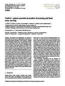
Figure 1. Selected basins.
sonal forecasts, dynamical modeling is thought to hold the greatest potential for future improvement in reliable seasonal streamflow forecasting (Zwiers and von Storch, 2004). Dynamical model experiments involve the integration of general circulation models (GCMs), which model atmospheric, oceanic and land surface interactions and processes as a set of dynamic equations. Seasonal forecasting by GCMs is based on coupled ocean–atmospheric integrations, where both atmospheric and oceanic components of the Earth’s system are taken into account. The main source of predictability for climate forecasting at seasonal scale is the long-term predictability of the oceanic circulation and its large impact on the global atmospheric circulation. The most important cause of seasonal climate variability is the ENSO (El Niño– Southern Oscillation) cycle, which is the large-scale fluctuation of ocean temperatures, rainfall, atmospheric circulation, vertical motion and air pressure centered over the tropical Pacific but affecting other ocean basins as well. Similarly, unusually warm or cold sea surface temperatures (SST) in other tropical oceans, the extent and thickness of snow cover and the amount of soil moisture can have a persistent influence on the atmospheric circulation (Persson and Grazzini, 2007). Due to the chaotic nature of the atmospheric–oceanic system, model runs made with small, random perturbations in the input data may produce a wide range of difference in the output. Therefore, GCMs are run multiple times with slightly different sets of initial conditions, producing a set of output data called an ensemble. The hydrological output from the land surface scheme of a GCM may be used as streamflow forecasts. Alternatively, the meteorological forecast ensemble by a GCM may be used as input to a hydrological model,
Hydrol. Earth Syst. Sci., 21, 4103–4114, 2017
which produces streamflow forecast ensembles, as we do in this research. This paper investigates the skill of seasonal streamflow forecasts for 20 of the largest rivers in the world with the global hydrological forecasting system Flood Early Warning System (FEWS)-World, which has been set up within the European Commission 7th Framework Programme Project Global Water Scarcity Information Service (GLOWASIS). These 20 rivers have been selected for analysis to represent different hydroclimatic conditions and all continents. Selected basins can be seen in Fig. 1; gauging stations and basin characteristics are summarized in Table 1. FEWS-World incorporates the global hydrological model PCR-GLOBWB (PCRaster Global Water Balance). The capability of global hydrological models to predict streamflow was demonstrated previously by several studies such as the WaterGap (Alcamo et al., 2003; Döll et al., 2003), LaD (Milly and Schmakin, 2002), VIC (Nijssen et al., 2001), WBM (Vörösmarty et al., 2000; Fekete et al., 2002), MacroPDM (Arnell, 1999, 2004) and PCR-GLOBWB (SpernaWeiland et al., 2010; van Beek et al., 2011). Candogan Yossef et al. (2012) assessed the skill of the global hydrological model PCR-GLOBWB in reproducing past discharge extremes for 20 large rivers of the world, as a first step towards developing a global seasonal hydrological forecasting system and assessing its skill. The study quantified skill in deterministic hindcast mode, using the ERA-40 reanalyses by the European Centre for Medium-range Weather Forecasts (ECMWF). This preliminary assessment by Candogan Yossef et al. (2012) concluded that the prospects for seasonal forecasting with PCR-GLOBWB or comparable models are positive. Since actual probabilistic meteorological forecast
www.hydrol-earth-syst-sci.net/21/4103/2017/
N. Candogan Yossef et al.: Skill of a global forecasting system
4105
Table 1. Basin characteristics and gauging stations (GRDC). Basin
Gauging station
Amazon Parana Brahmaputra Yangtze Yellow River Mekong McKenzie Nelson Ob Lena Rhine Danube Volga Columbia St. Lawrence Mississippi Murray–Darling Orange River Zambezi Nile
Obidos Corientes Bahadurabad Datong Huayuankou Muhdahan ArcticRedRiver Kettle Generating Station Salekhard Kyusur Rees Ceatal Izmail Volgograd Power Plant Beaver Army Terminal Cornwall Vicksburg Lock 9 Upstream Vioolsdrif Lukulu El Ekhsase
ensembles were not used, the assessment did not include errors in the meteorological forcing. However, in an actual forecasting setup, the predictive skill of a hydrological forecasting system is affected not only by errors in model structure and parameterization and initial conditions such as soil moisture, groundwater and snow, but also by meteorological forcing errors. Skill of seasonal hydrological forecasts can thus be improved by better meteorological forecasts on the one hand and by better estimation of initial hydrologic states through assimilation of independent hydrological observations on the other hand. The improvement in the overall predictability that may be attained depends on the relative importance of these two sources of uncertainty, which varies considerably among hydrological systems according to location, season and lead time (Bierkens and van den Hurk, 2007; Bierkens and van Beek, 2009; Shukla and Lettenmaier, 2011; Shukla et al., 2011; Yuan et al., 2015). Candogan Yossef et al. (2013) assessed the roles of initial conditions (ICs) and meteorological forcing (MF) in the skill of the global seasonal streamflow forecasting system FEWS-World, based on the ESP/revESP procedure outlined by Wood and Lettenmaier (2008). This study shows the potential for improvement in the skill of streamflow forecasts by a better estimation of IC or a more accurate MF input per region and per time of the year. The current paper aims to assess the total skill of hydrological forecasts, as affected by errors in model structure, in the estimation of IC as well as in the actual meteorological forecasts that are used to force the model.
www.hydrol-earth-syst-sci.net/21/4103/2017/
Area (km2 )
Qavg (m3 s−1 )
6 915 000 2 583 000 930 000 1 800 000 752 000 795 000 1 660 000 1 060 000 2 950 000 2 430 000 65 700 817 000 1 360 000 665 400 774 000 2 981 000 991 000 866 500 206 530 2 900 000
190 000 18 000 48 160 31 900 2570 16 000 9213 3447 12 680 17 000 2200 6400 8115 6670 7367 12 740 257 259 776 1251
The remaining part of this paper is set up as follows. Section 2 describes the global seasonal hydrological forecasting system, FEWS-World, the global hydrological model PCRGLOBWB, the meteorological forcing data, the hydrological simulations and the skill assessment. Results are presented in Sect. 3, followed by discussion in Sect. 4 and conclusions in the last section.
2 2.1
Materials and methods Global hydrological forecasting system FEWS-World
FEWS-World is a global hydrological forecasting system configured within the forecasting environment Delft-FEWS. Delft-FEWS is an open shell for data handling, managing and guiding forecasting processes (Werner et al., 2013). It is used by a large number of operational forecasting centers and agencies around the world for various purposes such as forecasting hydrological storm surges, river flows, reservoir management and water quality. FEWS-World has been built as part of the GLOWASIS project. The FEWS-World system consists of a master controller, a Postgres database and 18 forecasting shells (i.e., computational cores) for efficient handling of ensemble forecasts and data processing. Within FEWS-World several workflows have been set up for running the global hydrological model PCR-GLOBWB using the precipitation, temperature and potential evaporation fields from the ERA-Interim/Land GPCP-corrected dataset (Balsamo et Hydrol. Earth Syst. Sci., 21, 4103–4114, 2017
4106
N. Candogan Yossef et al.: Skill of a global forecasting system
al., 2015). Further descriptions of the meteorological forcing datasets are given in Sect. 2.2. PCR-GLOBWB simulates the terrestrial part of the global water cycle (van Beek et al., 2011; van Beek and Bierkens, 2009). It is coded in the high-level computer language PCRaster for constructing environmental models (Wesseling et al., 1996). The model is fully distributed and operates on a regular grid with a cell size of 0.5◦ × 0.5◦ on a daily time step. Meteorological forcing is assumed to be constant over the grid cell. Sub-grid variability of hydrological processes is taken into account in the representation of short and tall vegetation, open water, different soil types, saturated area, surface runoff, interflow and groundwater discharge. PCR-GLOBWB calculates the water balance for every grid cell by tracking the transfer of water between the atmosphere and the cell, through stores within each cell, and laterally, as discharge, from one cell to the downstream neighbor. The model calculates the storages and fluxes of water, and simulates the generation of runoff and its propagation as discharge through the river network. Precipitation falls either as snow or rain depending on atmospheric temperature. It can be intercepted by vegetation and added to the finite canopy storage, which is subject to open-water evaporation. Snow is accumulated when the temperature is lower than 0 ◦ C and melts when it is higher. Snowmelt is added to rain and throughfall; it is either stored in the available pore space in the snow cover, or it infiltrates into the top soil layer. Part of this water is transformed into surface runoff and the remainder infiltrates into the soil through two vertically stacked soil layers and an underlying groundwater layer. Water is exchanged between these layers following Darcy’s law and the resulting soil moisture is subject to evapotranspiration. The remaining water contributes to lateral drainage as interflow from the soil layers or baseflow from the groundwater reservoir. The total drainage, consisting of surface runoff, interflow and baseflow, is routed through the drainage network of rivers, lakes, wetlands and reservoirs, using the kinematic wave approach, based on the global drainage direction map DDM30, which describes the drainage directions of surface water with a spatial resolution of 300 longitude by 300 latitude (Döll and Lehner, 2002). An extensive description of PCRGLOBWB can be found in van Beek and Bierkens (2009). 2.2
Meteorological forcing data
The meteorological variables required to force PCRGLOBWB are daily values of precipitation, evapotranspiration and temperature. In the absence of direct estimates of actual evapotranspiration, the model can be forced with values of reference potential evapotranspiration, calculated from temperature, radiation, cloud cover, vapor pressure and wind speed. We force PCR-GLOBWB with two different datasets. The first one is the ERA-Interim/Land dataset (Balsamo et al., 2015). This is a global meteorological dataset, which is Hydrol. Earth Syst. Sci., 21, 4103–4114, 2017
a combination of the ERA-Interim reanalysis (Dee et al., 2011) and Global Precipitation Climatology Project (GPCP) monthly rainfall observations (Huffman and Bolvin, 2011; Huffman et al., 2009). ERA-Interim is a robust global atmospheric reanalysis produced by the ECMWF. It is an “interim” reanalysis initially started from the year 1989; later extended back to the year 1979, and continues to be updated forward in time. ERA-Interim reanalysis was produced as a part of the next-generation extended reanalysis intended to replace ERA-40. The GPCP is part of the Global Energy and Water Cycle Experiment (GEWEX) of the World Climate Research program (WCRP). The GPCP provides global precipitation estimates by merging infrared and microwave satellite estimates with rain gauge data from more than 6000 stations. Monthly values of potential evaporation have been estimated from ERA-Interim, using fields of temperature, radiation, cloud cover, vapor pressure and wind speed, by application of the Penman–Monteith equation (Monteith, 1981; Penman, 1948) for a reference grass canopy, according to the FAO methodology (Allen et al., 1998). Reference potential evaporation is multiplied by a monthly crop factor to obtain land cover specific potential evaporation in PCR-GLOBWB. The second dataset that we use to force the model is the re-forecast ensemble of the system-3 (S3) seasonal forecast archives of the ECMWF covering the period 1981–2010. S3 seasonal forecasts are run in ensemble mode on a fully coupled ocean–atmosphere model. They are run on the first of every month as the initial date, integrated forward for 6 months. Verifications show that the skill of forecasts in regions and seasons known to have a teleconnection with the El Niño is much higher than during neutral conditions. ECMWF seasonal forecast system has been shown to be superior to statistical systems in forecasting the onset of El Niño or La Niña. But once an event has started statistical systems have comparable skill. The dynamical model is also better than the statistical models in forecasting the SST in the Atlantic Ocean and the Indian Ocean. In many parts of the tropics, where changes such as those associated with El Niño can have a large impact on global weather patterns, a substantial part of the year-to-year variation in seasonal-mean rainfall and temperature is predictable. In mid-latitudes, the level of predictability is lower and Europe, in particular, is a difficult area to predict. Seasonal forecasts start to show signs of systematic model errors after about 10 days into the forecast. The ECMWF does not introduce any artificial terms in the equations to reduce the drift. Rather, a daily bias correction based on quantile–quantile transformation is applied on each forecast. In order to account for drift, we applied a bias correction using datasets varying per forecast month. As a result, there are 12 bias correction datasets each with a length equal to a seasonal forecast. The bias correction dataset was provided by the ECMWF (Emanuel Dutra, personal communication, 2015) within the GLOWASIS project. Since November 2011 the seasonal forecast system S4 has become operational to replace S3 with the goal of improving those aswww.hydrol-earth-syst-sci.net/21/4103/2017/
N. Candogan Yossef et al.: Skill of a global forecasting system pects, where S3 had problems. The improvements brought by S4 include, a next-generation ocean model, a higher spatial resolution, a larger ensemble size. The ensemble number of re-forecasts, which is relevant to our study, was increased from 11 to 15, and the forecasts integrated forward for 7, instead of 6 months. Though there are not many published references on S4 yet, initial studies indicate that there are some improvements in performance over S3, such as higher skill for ENSO forecasts. However, there are also certain aspects where the performance is worse. For instance, S4 suffers from a stronger bias in tropical Pacific SST than S3 (Molteni et al., 2011). Concerning the skill of re-forecast ensembles, an initial report by Norton and Rowlands (2011) compares the skill of 15-member S4 re-forecasts, to the 11-member S3 re-forecasts for the period 1981–2010; and concludes that there is no clear separation in skill between S3 and S4 on seasonal forecast timescales, from month 2 onwards. Therefore, taking into consideration that temperature and precipitation from the S3 re-forecast ensembles were bias corrected, we conclude that S3 is the preferred dataset for our study. 2.3
Streamflow forecast runs
PCR-GLOBWB is run at a daily time step to produce two sets of streamflow forecast ensembles, as well as the control simulation run. The first forecast run follows the ESP procedure using the ERA-Interim/Land dataset as basis for the meteorological input. The second forecast run uses actual ECMWF S3 seasonal forecasts as meteorological input. Model spin-up is carried out over the period 1979–1984 using ERA-Interim/Land dataset. Subsequently, the hydrological states at the end of this 5-year spin-up are used as initial states for the control run. The control run started from these initial states with the ECMWF S3 seasonal forecasts for the period 1979–2010. Daily discharge values are aggregated into monthly totals. Monthly aggregation provides a more appropriate forecast at the seasonal scale and a proxy of the underlying distribution. Hydrologic states, as well as monthly discharge totals, are saved at the end of each month. These states are used as ICs for running the ESP as well as the ECMWF S3 seasonal forecasts. The ESP forecast ensemble is produced with the ESP workflow within Delft-FEWS. Input ensembles of the meteorological forcing are created from the 32-year input data series (1979–2010). PCR-GLOBWB model runs are initialized on the first day of each month using the stored ICs. In order to avoid any further bias, we excluded the first 2 years and limited the subsequent analysis to the period 1981–2010. This results in 360 ESP runs, each run containing 31 members, excluding the year in question from the 32-year series. The ECMWF S3 streamflow forecast ensemble is produced by forcing the model with bias-corrected meteorological input dataset from the ECMWF S3 seasonal forecast archive, containing 11 ensemble members for each forecast and covering the period 1981–2010. (12 monthly forecasts over the www.hydrol-earth-syst-sci.net/21/4103/2017/
4107 30-year period result in 30×12 = 360 runs, with 11 ensemble members for each run.) Both the ESP and ECMWF S3 runs are carried out in batch using the FEWS-World forecasting system. Each run spans 6 months and produces an ensemble of 11 monthly discharge values for six lead times. 2.4
Skill assessment
The Brier skill score (BSS) is commonly used for the skill assessment of meteorological probabilistic forecasts. In order to quantify the added skill obtained by using ECMWF S3 seasonal meteorological forecasts compared to the reference ESP forecast, we employ the BSS, calculated by Eq. (1): BSS = 1 −
BSforecast . BSref
(1)
The BS values for a given month and lead time are given by Eq. (2): BS =
N 1 X (pt − ot )2 , N t=1
(2)
where N is the number of forecasting instances, p is the forecasted probability and o is the observed probability. The range of the BSS is (−∞, 1) and the best value for a perfect forecast is 1. When the BSS is equal to 0, the forecast skill is equal to that of the reference forecast. Here, a skill of zero or less implies that the seasonal forecasts provide no additional information compared to the random generated climatology of the ESP forecast run. The range of the BS is (0, 1), 0 being the best value for a perfect forecast and 1 the worst. Besides the BS and its associated skill score BSS, it is possible to use other verification metrics, such as the relative operating characteristic (ROC) score, or the continuous ranked probability skill score (CRPSS) for the skill assessment. We prefer to use the BS and BSS since we would like to assess the skill of our forecasting system in predicting a category of high, low or normal flow for the given month, rather than an exact discharge value, and BS is very suitable for this purpose. BS is the mean squared error of probabilistic forecasts for a given dichotomous event. A probability threshold is used to define the binary event to be observed and forecasted. The BS is a relevant verification metric for analyzing the performance of a forecast system for specific categories, defined by a set of thresholds. It is preferred for being a proper score, i.e., being optimized for forecasts that correspond to the best judgment of the forecaster. It is also a highly compressed score; i.e., it directly accounts for forecast probabilities without necessitating a contingency table for each probability threshold (Bartholmes et al., 2009; Ferro, 2007). In this study, we use two probability thresholds corresponding to the 25th and 75th percentiles for high and low flows, respectively. Values below the 25th percentile of a Hydrol. Earth Syst. Sci., 21, 4103–4114, 2017
4108
N. Candogan Yossef et al.: Skill of a global forecasting system
Table 2. Meteorological datasets used for calculating BS. Theoretical (BStheo )
BSforecast BSref
forecasted (p)
observed (o)
forecasted (p)
observed (o)
ECMWF S3 ESP
ERA 40 ERA 40
ECMWF S3 ESP
GRDC GRDC
given month of the year are considered low flows and those above the 75th percentile are considered high flows. The thresholds are calculated separately for forecasted values and observed values. In other words, we classify a forecasted value as high flow if it exceeds the 75th percentile of all forecasted values for the same month of the year and low flow if it is below the 25th percentile. Similarly, an observed value is classified as high flow if it exceeds the 75th percentile of all observed values for the same month of the year and low flow if it is below the 25th percentile. This approach eliminates any systematic bias in the simulations compared to the observations. In this way, we are able to assess the skill in forecasting the occurrence of flows that are higher or lower than usual for a given month. We calculate the BS and BSS values in 20 large global basins separately for the 12 months of the year and for all six lead times. When calculating the BS for a given month and a given lead time, we use the forecast ensembles that predict the total monthly discharge generated during that given month. In other words, we use the discharge ensembles resulting from the simulations that start at time t0 and end at time tn with a lead time of n months, where t0 is prior to the end of the given forecast month by n months. Thus, for the month of May and for a 1-month lead time, n = 1, t0 is 1 May and tn is 31 May. For a 2-month lead time, n = 2, t0 is 1 April and tn is again the 31 May. For the ESP approach and the ECMWF S3 seasonal meteorological forecasts, we quantify the theoretical as well as the actual skill. To calculate the theoretical skill, we compare the ESP and ECMWF S3 streamflow forecast ensembles to the results of the control simulation; and for the actual skill we compare them to observed discharge records. The discharge records used are provided by the Global Runoff Data Centre (GRDC) and measured at stations located at the basin outlets. The meteorological datasets used in the calculation of scores are clarified in Table 2.
3 3.1
Actual (BSact )
Results Skill scores
We present the results of the skill assessment in 20 score tables for 20 rivers (Tables S1–S20). The tables are presented in the Supplement. The first eight parts of each table show the BS values for the ECMWF S3 forecast as well as the Hydrol. Earth Syst. Sci., 21, 4103–4114, 2017
BSS values, calculated for the four cases of actual and theoretical skill, for low and high flows, i.e., the 25th and the 75th percentiles. Tables present the scores for the 12 months of the year and for six lead times. The tables are color coded for easier visual inspection. Values are highlighted in blue where the accuracy of the ECMWF S3 forecasts is considerably higher than that of the ESP forecast, and in yellow where it is considerably lower. Since the best value for BS is 0, higher forecast accuracy corresponds to a lower BS. Where the difference between the BS values of the ECMWF S3 and ESP forecasts are larger or equal to 0.05, the value is highlighted in light blue or light yellow; where it is larger or equal to 0.1, it is highlighted in dark blue or dark yellow. The last two parts of each table show the ratios of the BSact to BStheo of both the ESP and ECMWF S3 forecasts, for the 12 months of the year and six lead times, for low and high flows, respectively. 3.2
Overview of the basins with added skill
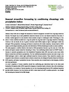
We provide a global overview of the basins where added skill is obtained using ECMWF S3 meteorological forecast input compared to the ESP input. The locations of improved skill are presented on four world maps for the four cases of actual and theoretical skill, for low and high flows, i.e., the 25th and the 75th percentiles (Fig. 2). The maps indicate the number of months per year with skillful forecasts at each location, as well as the maximum lead time for which the skill is retained. 4
Discussion of results
In this section, we discuss the results for several larger basins in the context of prevailing hydroclimatic conditions. 4.1
Tropical, monsoon-dominated basins
As can be seen in Fig. 2a, results indicate that in the Amazon basin the theoretical skill of the ECMWF S3 forecasts is quite high for predicting lower flows than usual for the given month. In Table S1 for the Amazon, the color-coded first part, which presents the BStheo for low flow, shows that most of the values are colored blue. This indicates that the accuracy of ECMWF S3 forecasts are significantly higher than the ESP forecasts; i.e., the difference between the BS values is higher than 0.05. For lead times of 1 and 2 months, the improvement is larger, as can be seen on the first two columns, www.hydrol-earth-syst-sci.net/21/4103/2017/
N. Candogan Yossef et al.: Skill of a global forecasting system
4109
Figure 2. Global overview of basins with improved forecast skill. Panels (a) theoretical skill in low flows, (b) theoretical skill in high flows, (c) actual skill in low flows, (d) actual skill in high flows.
www.hydrol-earth-syst-sci.net/21/4103/2017/
Hydrol. Earth Syst. Sci., 21, 4103–4114, 2017
4110 which are colored mostly dark blue, indicating a difference between BS values higher than 0.1. The results for high flows are very different than those for low flows, as can be seen in Fig. 2b, as well as the third and fourth parts of Table S1. Most BS values of the ECMWF S3 are very close to the ESP, with only a few yellow highlighted values denoting a worse performance. The results are also different for the actual skill as can be seen in Fig. 2c and d. Both for low and high flows (the fifth to eighth parts of the Table S1), the performance of the ECMWF S3 is either very close to the ESP or lower, as can be seen again by the yellow color. The average ratio of BSact to BStheo of the ECMWF S3 forecasts over the year and the six lead times is 0.5 in forecasting low flows and 0.57 in high flows (the last two parts of Table S1). These ratios increase with increasing lead time, starting from 0.21 for low flows at a lead time of 1 month, and rising to 0.68 at a lead time of 6 months. There are considerable differences in the ratios between months as well. Candogan Yossef et al. (2012) showed that hydrological forecasting skill in the Amazon basin is dominated by initial conditions for lead times of 1–2 months, and even up to 4 months for forecasting the discharge during the Southern Hemisphere spring, from August until November. Initial conditions are especially important during high-flow conditions (March, April and May) (Paiva et al., 2012) and the recession period (June, July, August), when the increased groundwater storage plays an important role. Moreover, in large basins such as the Amazon where long travel times are involved, the knowledge of surface water conditions several months ahead is an important source of forecast skill. Meteorological forcing starts to play a more important role beyond 1–2-month lead times throughout the rest of the year. The present study shows, however, that by using ECMWF S3 seasonal forecasts the biggest skill improvement over the ESP procedure can be attained at lead times of 1–2 months, but less at longer lead times when meteorological forcing plays a more important role. For lead times beyond 1–2 months an improvement in skill during most of the year still exists, but it should be noted that this improvement is observed only in the theoretical skill in forecasting low flows. The results for the other tropical South American basin that we study, the Parana, shows a somewhat similar pattern to the Amazon, in the sense that the theoretical skill of ECMWF S3 in forecasting low flows is higher than ESP in some cases, whereas for high flows it is mostly lower (see Table S2). In contrast, the actual skill of ECMWF S3 in forecasting both high and low flows in the Parana is quite different than that in the Amazon. The ratio of actual to theoretical skill of ECMWF S3 forecasts is much lower than that in the Amazon. Averaged over the months of the year and different lead times, it is 0.27 and 0.25 for low and high flows, respectively. Notwithstanding, comparing the actual skill of the ECMWF S3 forecasts to the ESP, we see several months and lead times where the actual skill is significantly improved by Hydrol. Earth Syst. Sci., 21, 4103–4114, 2017
N. Candogan Yossef et al.: Skill of a global forecasting system using ECMWF S3 forecasts, especially for forecasting high flows at longer lead times and during the first half of the year. For shorter lead times and for the second half of the year however, the actual performance of ECMWF S3 in forecasting high flows is significantly worse than ESP. In forecasting low flows, forecast accuracy is also mostly reduced by using ECMWF S3 forecasts. Another monsoon-dominated tropical river, the Brahmaputra in the Indian sub-continent, shows a similar pattern to the Parana. In Table S3, we see again a significant improvement in the actual skill for forecasting high flows at longer lead times during the first half of the year. Just like the Parana, forecast accuracy is significantly lower at shorter lead times during the second half of the year. In contrast, the actual skill for forecasting low flows is significantly low at longer lead times, and high at a lead time of 1 month. In theoretical skill, the accuracy of ECMWF S3 re-forecasts in the Brahmaputra for both high and low flows is either very close to that of the ESP or lower. The ratio of the theoretical skill of ECMWF S3 to the actual skill varies considerably for high and low flows, as well as over the year and the range of lead times. The averages are 0.24 and 0.34 for low and high flows, respectively, ranging from as low as 0.2 for low flow forecasts in January to as high as 1.25 for high-flow forecasts in April. The BS values for April high flows at all lead times are higher for actual skill calculations where the forecasted discharges are compared to actual discharge records, than the theoretical skill where they are compared to model simulations. Indeed, it was shown by Candogan Yossef et al. (2012) that the ESP procedure performs worse than the unconditional climatological record of observed flow from April to September even for lead times of 1 month. The forecast skill in the Brahmaputra is strongly dominated by MF during the monsoon season for all lead times. During these months, at a lead time of 1 month, the ECMWF S3 performs significantly worse than the ESP, for the assessment of actual skill. This means the apparent potential for improvement in hydrological forecasts at short lead times by using ECMWF S3 seasonal meteorological forecasts cannot be realized at the moment. In the two large rivers of China, the Yangtze and the Yellow River, there exists a potential for improving forecasts beyond 1-month lead time through better MF during the high-flow period (see Table S4 and S5). This period extends from May to October in the Yellow River and from April to September in the Yangtze (Candogan Yossef et al., 2012). Our results for the actual skill in forecasting high flows show that this opportunity may be partly realized in both rivers. The added skill of ECMWF S3 over ESP in forecasting higher than usual discharges during the high-flow periods at longer lead times may aid the estimation of increased probability of flooding at lead times of 4–6 months. Moreover, the actual skill of ECMWF S3 is also high in forecasting low flows at short lead times during some months of the highflow periods, especially for the Yellow River. This may help a www.hydrol-earth-syst-sci.net/21/4103/2017/
N. Candogan Yossef et al.: Skill of a global forecasting system better estimation of the probability of less than expected discharges during high-flow periods, at 1–2-month lead times. The actual skill of ECMWF S3 forecasts in the Yangtze captures on average 0.23 of the theoretical skill for low flows, and 0.25 for high flows. These numbers are 0.22 and 0.26 in the Yellow River for low and high flows, respectively. In both rivers, for both high and low flows, a significant pattern emerges in the ratios of actual to theoretical skill. The ratios are considerably higher during wet periods than during dry periods. Similar to the Yellow River and the Yangtze, also in the Mekong basin forecast skill during the wet period from July to October is dominated by MF beyond 1-month lead time. However, the results for the Mekong are different from those for the Chinese basins. Added skill of ECMWF S3 over ESP in forecasting higher than usual discharges during the wet periods can be seen not at longer lead times, but only at a lead time of 1 month, as can be seen in Table S6. This may aid better estimation of flood probability at short notice. Beyond 1 month, the performance of ECMWF S3 forecasts are either worse or not significantly different than ESP. ECMWF S3 forecasts of lower than usual discharges during either the wet or dry periods perform worse than ESP at short lead times, but there are some months of improved skill at long lead times. The ratios of theoretical skill of ECMWF S3 forecasts to the actual skill in the Mekong are 0.37 and 0.60 for low and high flows, respectively. During the high-flow period from July to October, the actual skill in forecasting higher than usual discharges reaches more than 0.80 of the theoretical skill. 4.2
Arctic basins
In Arctic basins, snowpack, ice and groundwater processes have a long memory, causing the forecast skill to be dominated by ICs for lead times up to 6 months (Candogan Yossef et al., 2013). The North American Arctic rivers Mackenzie and Nelson, as well as the Asian Ob and Lena are ice bound for a significant part of the year and peak discharges follow snowmelt. The ESP forecasts already perform quite well in these Arctic rivers as would be expected for basin with such a large memory. Tables S7–S10 show that the ECMWF S3 forecasts for these rivers are not significantly skillful when compared to the ESP. During May–June, which is the beginning of the high-flow season in Arctic rivers, one might expect some improvement in skill with ECMWF S3 forecasts over the ESP due to the temperature effect determining the onset of snowmelt. However, there is no significant increase in the performance of ECMWF S3 forecasts over the ESP forecasts, not even during the beginning of the high-flow season. ECMWF S3 forecasts perform very similar to ESP, and even worse in some cases. Especially the actual skill of ECMWF S3 forecasts in the Arctic basins in Asia is considerably low when compared to the ESP forecasts. www.hydrol-earth-syst-sci.net/21/4103/2017/
4111 The ratios of actual skill to theoretical skill are not very low in the Arctic basins in general. Low ratios would be expected in areas where the model has large errors associated with snow and glaciers and consequent errors in the timing of peak discharges. In the river Ob for instance, where the discharge peaks in June, the actual skill reaches 0.60–0.70 of the theoretical skill, so it may be concluded that the timing of the model is well approximated. 4.3
Temperate regions
The ECMWF S3 forecasts in general do not perform significantly better than ESP in the temperate European basins, such as Rhine, Danube and Volga as can be seen in Tables S11–S13. There are some cases with improvement in the skill in forecasting flows lower than usual, especially in the theoretical skill. However, for high flows the ECMWF S3 forecasts perform worse than the ESP. In the Rhine basin, where improvement in forecast accuracy depends on better climate forecasts, using the ECMWF S3 forecasts does not provide an improvement over the ESP. In the Danube and the Volga, we see an improvement in the theoretical skill in forecasting low flows during winter months. In the Danube and especially the Volga basins snowmelt and groundwater processes play a bigger role than the Rhine. Low flows during winter months are actually dominated by the groundwater processes rather than the meteorological forcing. Nevertheless, this is where we see a consistent improvement in skill by using the ECMWF S3 forecasts. For high flows on the other hand, ECMWF S3 forecasts perform worse, both in their theoretical and actual skill. The ratios of actual to theoretical skill are in general quite high for the European basins, but lower in temperate basins of North America. In the Columbia River forecasts are dominated by the ICs due to snow and the performance of ESP forecasts is already high. Using ECMWF S3 forecasts does not bring a significant improvement (see Table S14). In the St. Lawrence River, peak flows are fed by spring and summer snowmelt accompanied by rain. Candogan Yossef et al. (2013) concluded that the forecasting skill in spring and summer months depends largely on the snowpack accumulated during the previous winter months, dominating seasonal forecasts up to 6 months ahead. These findings are in disagreement with the results of Shukla and Lettenmaier (2011), which show that ESP forecasts initialized from December to April are skillful only for 1–2-month lead times. As it was mentioned in Candogan Yossef et al. (2013), the disagreement is probably due to errors in one or both models in the estimation of snow accumulation. The results of the present study confirm the importance of ICs on the one hand. Table S15 shows that the theoretical skill of ECMWF S3 forecasts is considerably low compared to the ESP in the St. Lawrence, especially for forecasting higher flows than usual during the summer months. On the other hand, the actual skill of the ECMWF S3 forecasts in forecasting lower Hydrol. Earth Syst. Sci., 21, 4103–4114, 2017
4112
N. Candogan Yossef et al.: Skill of a global forecasting system
than usual summer flows is significantly high for 2, 3 and 4-month lead times. This finding supports the conclusion of Shukla and Lettenmaier (2011), which emphasizes the importance of MF beyond 1–2-month lead times. Additionally, the fact that the ratio of actual skill to theoretical skill in St. Lawrence is rather on the low side may be an indication of errors in our model in representing the snow processes. For the southeastern US rivers, the results of Candogan Yossef et al. (2013) as well as those of Shukla and Lettenmaier (2011) show that skill due to ICs diminishes after 1–2month lead time and that forecasts would benefit most from improvements in MF throughout the year. However, the results of the present study show that in general this potential improvement cannot be realized for the Mississippi by using ECMWF S3 forecasts. The performance of ECMWF S3 forecasts is similar to the ESP in most cases, as can be seen in Table S16, and it is lower than ESP in more case than it is higher, with no apparent pattern. 4.4
Semi-arid regions
Candogan Yossef et al. (2013) concluded that the relative importance of ICs is the lowest in the Murray–Darling basin and any improvement of hydrological forecasts depends on better climate forecasts. The results of the present study for this basin show that the theoretical skill of ECMWF S3 forecasts are significantly high in some cases, but lower in other cases, with no apparent pattern (see Table S17). The accuracy of ECMWF S3 forecasts in assessment of actual skill is lower than ESP in most cases. Also, the ratios of actual to theoretical skill are quite low in this basin for both high and low flows. Similarly, in the semi-arid African basins of the Orange River and the Zambezi, where the knowledge of MF plays a very important role in the forecast skill, the performance of ECMWF S3 forecasts is worse compared to the ESP in most cases. Tables S18 and S19 show that the accuracy of ECMWF S3 is lower than ESP in these basins, particularly in actual skill. In contrast, in the Nile basin, the ICs dominate the forecast skill, resulting in high performance of ESP forecasts throughout the year assuming that the release strategy of the Aswan reservoir is known (Candogan Yossef et al., 2013). The results of the present study show that the theoretical skill of ECMWF S3 cannot surpass the already high performance of the ESP (see Table S20). Actually, forecasts with ECMWF S3 perform considerably worse. In actual skill however, the accuracy of the ESP forecasts in the Nile is very low due to the large effect of the reservoir operations. In fact, the ratio of actual to theoretical skill is the lowest by far in this basin. With such a low accuracy of ESP forecasts despite the dominance of ICs, comparison of the performance of ECMWF S3 to ESP is not very meaningful. Our results of actual skill in both high and low flows in the Nile appear to be very erratic indeed.
Hydrol. Earth Syst. Sci., 21, 4103–4114, 2017
5
Conclusions
We assessed the skill of seasonal streamflow forecasts with the global hydrological forecasting system FEWS-World, set up within the GLOWASIS project. Global hydrological model PCR-GLOBWB was run with the ESP procedure as well as with ECMWF S3 bias-corrected seasonal meteorological forecast ensembles. We produced ensemble forecasts of monthly discharges for 20 large rivers of the world, with lead times of up to 6 months. We quantified the skill of ECMWF S3 forecasts compared to the reference ESP forecasts using the BSS, both for high and low flows. We determined the theoretical skill by comparing the results against model simulations, as well as the actual skill by comparing against discharge observations. We also calculated the ratios of actual to theoretical skill. We analyzed these results in the context of prevailing hydroclimatic conditions. This analysis suggests that the skill varies considerably according to location, season and lead time. The conclusions can be summarized as follows: – In general, the performance of the ECMWF S3 forecast run is close to that of the ESP forecast run. – There are basins where the ECMWF S3 forecast run performs significantly better than the ESP, during certain periods of the year and at certain lead times. – However, there are in fact more cases where the ECMWF S3 forecast run performs worse than the ESP. – In most cases, the apparent potential for improvement in seasonal hydrological forecasts by using better meteorological forecasts cannot be realized as yet with the model PCR-GLOBWB and the ECMWF S3 re-forecast dataset. – As more accurate global hydrological models and more skillful seasonal meteorological forecasts become available in the future, such as the most recent ECMWF system S4, further studies will be needed to assess the improvement in seasonal hydrological forecasts, as well as the effect of meteorological forecast quality vs. model errors on the hydrological forecasts.
Data availability. Available research data are presented in the Supplement.
The Supplement related to this article is available online at https://doi.org/10.5194/hess-21-4103-2017supplement.
Competing interests. The authors declare that they have no conflict of interest.
www.hydrol-earth-syst-sci.net/21/4103/2017/
N. Candogan Yossef et al.: Skill of a global forecasting system Acknowledgements. The forecast system, used in this research, has been set up in the 7th Framework Programme Project Global Water Scarcity Information Service (GLOWASIS). We acknowledge the 7th Framework Programme of the European Commission for the financial support. Furthermore, we acknowledge the European Centre for Medium-ranged Weather Forecasts for making available the ERA Interim – GPCP dataset and the ECMWF S3 seasonal forecasts ensemble used in this study as meteorological forcing. We also acknowledge and thank Emanuel Dutra personally for providing the bias correction datasets. Edited by: Maria-Helena Ramos Reviewed by: three anonymous referees
References Alcamo, J., Döll, P., Henrichs, T., Kaspar, F., Lehner, B., Rösch, T., and Siebert, S.: Development and testing of the WaterGAP 2 global model of water use and availability, Hydrol. Sci. J., 48, 317–337, https://doi.org/10.1623/hysj.48.3.317.45290, 2003. Allen, R. G., Pereira, L. S., Raes, D., and Smith, M.: Crop evapotranspiration, FAO Irrig. Drain. Pap. 56, Food and Agric. Organ., Rome, 1998. Arnell, N. W.: A simple water balance model for the simulation of streamflow over a large geographic domain, J. Hydrol., 27, 314– 335, 1999. Arnell, N. W.: Climate change and global water resources: SRES emissions and socio-economic scenarios, Global Environ. Change, 14, 31–52, https://doi.org/10.1016/j.gloenvcha.2003.10.006, 2004. Balsamo, G., Albergel, C., Beljaars, A., Boussetta, S., Brun, E., Cloke, H., Dee, D., Dutra, E., Muñoz-Sabater, J., Pappenberger, F., de Rosnay, P., Stockdale, T., and Vitart, F.: ERAInterim/Land: a global land surface reanalysis data set, Hydrol. Earth Syst. Sci., 19, 389–407, https://doi.org/10.5194/hess-19389-2015, 2015. Bartholmes, J. C., Thielen, J., Ramos, M. H., and Gentilini, S.: The european flood alert system EFAS – Part 2: Statistical skill assessment of probabilistic and deterministic operational forecasts, Hydrol. Earth Syst. Sci., 13, 141–153, https://doi.org/10.5194/hess-13-141-2009, 2009. Bierkens, M. F. P. and van Beek, L. P. H.: Seasonal predictability of European discharge: NAO and hydrological response time, J. Hydrometeorol., 10, 953–968, 2009. Bierkens, M. F. P. and van den Hurk, B. J. J. M.: Groundwater convergence as a possible mechanism for multi-year persistence in rainfall, Geophys. Res. Lett., 34, LO2402, https://doi.org/10.1029/2006GL028396, 2007. Candogan Yossef, N., van Beek, L. P. H., Kwadijk, J. C. J., and Bierkens, M. F. P.: Assessment of the potential forecasting skill of a global hydrological model in reproducing the occurrence of monthly flow extremes, Hydrol. Earth Syst. Sci., 16, 4233–4246, https://doi.org/10.5194/hess-16-4233-2012, 2012. Candogan Yossef, N., Winsemius, H., van Beek, L. P. H., Weerts, A., and Bierkens, M. F. P.: Skill of a global seasonal streamflow forecasting system, relative roles of initial conditions and meteorological forcing, Water Resour. Res., 49, 4687–4699, https://doi.org/10.1002/wrcr.20350, 2013.
www.hydrol-earth-syst-sci.net/21/4103/2017/
4113 Dee, D. P., Uppala, S. M., Simmons, A. J., Berrisford, P., Poli, P., Kobayashi, S., Andrae, U., Balmaseda, M. A., Balsamo, G., Bauer, P., Bechtold, P., Beljaars, A. C. M., van de Berg, I., Biblot, J., Bormann, N., Delsol, C., Dragani, R., Fuentes, M., Greer, A. J., Haimberger, L., Healy, S. B., Hersbach, H., Holm, E. V., Isaksen, L., Kallberg, P., Kohler, M., Matricardi, M., McNally, A. P., Mong-Sanz, B. M., Morcette, J.-J., Park, B.-K., Peubey, C., de Rosnay, P., Tavolato, C., Thepaut, J. N., and Vitart, F.: The ERAInterim reanalysis: Configuration and performance of the data assimilation system, Q. J. Roy. Meteorol. Soc., 137, 553–597, 2011. Döll, P. and Lehner, B.: Validating of a new global 30-minute drainage direction map, J. Hydrol., 258, 214–231, 2002. Döll, P., Kaspar, F., and Lehner, B.: A global hydrological model for deriving water availability indicators: model tuning and validation, J. Hydrol., 270, 105–134, 2003. Fekete, B. M., Vörösmarty, C. J., and Grabs, W.: High-resolution fields of global runoff combining observed river discharge and simulated water balances, Global Biogeochem. Cy., 16, 1042, https://doi.org/10.1029/1999GB001254, 2002. Ferro, C. A. T.: Comparing probabilistic forecasting systems with the brier score, Weather Forecast., 22, 1089–1100, https://doi.org/10.1175/WAF1034.1, 2007. Huffman, G. J. and Bolvin D. T.: GPCP Version 2.2 Combined Precipitation Data Set Documentation, available at: ftp://precip.gsfc. nasa.gov/pub/gpcp-v2.2/doc/V2.2_doc.pdf, 2011. Huffman, G. J., Adler, R. F., Bolvin, D. T., and Gu, G.: Improving the Global Precipitation Record: GPCP Version 2.1, Geophys. Res. Lett., 36, L17808, https://doi.org/10.1029/2009GL040000, 2009. Milly, P. C. D. and Schmakin, A. B.: Global modelling of land water and energy balances, Part I: the land dynamics (LaD) model, J. Hydrometeorol., 3, 283–299, 2002. Molteni, F., Stockdale, T., Balmaseda, M., Balsamo, G. Buizza, R., Ferranti, L., Magnusson, L., Mogensen, K., Palmer, T., and Vitart, F.: The new ECMWF seasonal forecast system (System 4), available at: http://www.ecmwf.int/sites/default/files/elibrary/2011/ 11209-new-ecmwf-seasonal-forecast-system-system-4.pdf, 2011. Monteith, J. L.: Evaporation and surface temperature, Q. J. Roy. Meteor. Soc., 107, 1–27, 1981. Nijssen, B., O’Donnell, G. M., Lettenmaier, D. P., Lohmann, D., and Wood, E. F.: Predicting the discharge of global rivers, J. Climate, 14, 3307–3323, 2001. Norton, W. and Rowlands, D.: First impressions of seasonal forecasting system 4, available at: http://www.ecmwf.int/sites/default/files/elibrary/2011/ 14898-first-impressions-seasonal-forecasting-system-4.pdf, 2011. Paiva, R. C. D., Collischonn, W., Bonnet, M. P., and de Gonçalves, L. G. G.: On the sources of hydrological prediction uncertainty in the Amazon, Hydrol. Earth Syst. Sci., 16, 3127–3137, https://doi.org/10.5194/hess-16-3127-2012, 2012. Penman, H. L.: Natural evaporation from open water, bare soil, and grass, P. Roy. Soc. Lond. A Mat., 193, 120–145, https://doi.org/10.1098/rspa.1948.0037, 1948.
Hydrol. Earth Syst. Sci., 21, 4103–4114, 2017
4114 Persson, A. and Grazzini, F.: User Guide to ECMWF forecast products, available at: http://old.ecmwf.int/products/forecasts/guide/ index.html, 2007. Shukla, S. and Lettenmaier, D. P.: Seasonal hydrologic prediction in the United States: understanding the role of initial hydrologic conditions and seasonal climate forecast skill, Hydrol. Earth Syst. Sci., 15, 3529–3538, https://doi.org/10.5194/hess-153529-2011, 2011. Shukla, S., Sheffield, J., Wood, E. F., and Lettenmaier, D. P.: Relative contributions of initial hydrologic conditions and seasonal climate forecast skill to seasonal hydrologic prediction globally, 2011 Fall Meeting, AGU, San Francisco, California, 5–9 December 2011, H51N-05, 2011. Sperna Weiland, F. C., van Beek, L. P. H., Kwadijk, J. C. J., and Bierkens, M. F. P.: The ability of a GCM-forced hydrological model to reproduce global discharge variability, Hydrol. Earth Syst. Sci., 14, 1595–1621, https://doi.org/10.5194/hess-14-15952010, 2010. Van Beek, L. P. H. and Bierkens M. F. P.: The Global Hydrological Model PCR-GLOBWB: Conceptualization, parameterization and verification, Report, Department of Phys. Geogr., Utrecht Univ., Utrecht, Netherlands, available at: http://vanbeek.geo.uu. nl/suppinfo/vanbeekbierkens2009.pdf, 2009. Van Beek, L. P. H., Wada, Y., and Bierkens, M. F. P.: Global monthly water stress: I. Water balance and water availability, Water Resour. Res., 47, W07517, https://doi.org/10.1029/2010WR009791, 2011.
Hydrol. Earth Syst. Sci., 21, 4103–4114, 2017
N. Candogan Yossef et al.: Skill of a global forecasting system Vörösmarty, C. J., Green, P., Salisbury, J., and Lammers R. B.: Global water resources: Vulnerability from climate change and population growth, Science, 289, 284–288, https://doi.org/10.1126/science.289.5477.284, 2000. Werner, M., Schellekens, J., Gijsbers, P., van Dijk, M., van den Akker, O., and Heynert, K.: The Delft-FEWS flow forecasting system, Environ. Modell. Softw., 40, 65–77, https://doi.org/10.1016/j.envsoft.2012.07.010, 2013. Wesseling, C. G., Karssenberg, D., van Deursen, W. P. A., and Burrough, P. A.: Integrating dynamic environmental models in GIS: the development of a Dynamic Modeling language, Transactions in GIS, 1, 40–48, 1996. Wood, A. W. and Lettenmaier, D. P.: An ensemble approach for attribution of hydrologic prediction uncertainty, Geophys. Res. Lett., 35, L14401, https://doi.org/10.1029/2008GL034648, 2008. Yuan, X., Wood, E. F., and Ma, Z.: A review on climatemodel-based seasonal hydrologic forecasting: physical understanding and system development, WIREs Water, 2, 523–536, https://doi.org/10.1002/wat2.1088, 2015. Zwiers, F. W. and von Storch, H.: On the role of statistics in climate research, Int. J. Climatol., 24, 665–680, 2004.
www.hydrol-earth-syst-sci.net/21/4103/2017/