Oct 8, 2010 - 2 â1-Norm Regularized/Constrained Problems. 10 ..... In the multi-class classification scenario with k > 2 classes, ..... Starting point: .x0, .c0, .init.
SLEP: Sparse Learning with Efficient Projections Version 4.0
Jun Liu, Shuiwang Ji, and Jieping Ye Computer Science and Engineering Center for Evolutionary Medicine and Informatics The Biodesign Institute Arizona State University Tempe, AZ 85287 {j.liu, shuiwang.ji, jieping.ye}@asu.edu http://www.public.asu.edu/˜jye02/Software/SLEP October 8, 2010
1
Contents 1 Introduction 1.1 Main Features . . . . . . . . . . . 1.2 How to Use the SLEP Package . . 1.3 Applicability of the SLEP Package 1.4 Folders & Examples . . . . . . .
. . . .
. . . .
. . . .
. . . .
. . . .
. . . .
. . . .
. . . .
. . . .
. . . .
. . . .
. . . .
. . . .
. . . .
. . . .
. . . .
. . . .
. . . .
4 6 7 8 8
2 ℓ1 -Norm Regularized/Constrained Problems 2.1 Euclidean Projection onto the ℓ1 Ball via Improved Bisection 2.2 LeastR . . . . . . . . . . . . . . . . . . . . . . . . . . . . . 2.3 LogisticR . . . . . . . . . . . . . . . . . . . . . . . . . . . 2.4 LeastC . . . . . . . . . . . . . . . . . . . . . . . . . . . . . 2.5 LogisticC . . . . . . . . . . . . . . . . . . . . . . . . . . . 2.6 nnLeastR . . . . . . . . . . . . . . . . . . . . . . . . . . . 2.7 nnLogisticR . . . . . . . . . . . . . . . . . . . . . . . . . . 2.8 nnLeastC . . . . . . . . . . . . . . . . . . . . . . . . . . . 2.9 nnLogisticC . . . . . . . . . . . . . . . . . . . . . . . . . .
. . . . . . . . .
. . . . . . . . .
. . . . . . . . .
. . . . . . . . .
. . . . . . . . .
. . . . . . . . .
. . . . . . . . .
. . . . . . . . .
. . . . . . . . .
. . . . . . . . .
. . . . . . . . .
. . . . . . . . .
. . . . . . . . .
. . . . . . . . .
. . . . . . . . .
. . . . . . . . .
. . . . . . . . .
10 10 11 12 13 13 14 15 15 16
. . . .
. . . .
. . . .
. . . .
. . . .
. . . .
. . . .
. . . .
. . . .
. . . .
. . . .
. . . .
. . . .
3 ℓ1 /ℓq -Norm Regularized Problems 3.1 The ℓq -Regularized Projection Via Bisection 3.2 glLeastR . . . . . . . . . . . . . . . . . . . 3.3 glLogisticR . . . . . . . . . . . . . . . . . 3.4 mtLeastR . . . . . . . . . . . . . . . . . . 3.5 mtLogisticR . . . . . . . . . . . . . . . . . 3.6 mcLeastR . . . . . . . . . . . . . . . . . . 3.7 mcLogisticR . . . . . . . . . . . . . . . . .
. . . . . . .
. . . . . . .
. . . . . . .
. . . . . . .
. . . . . . .
. . . . . . .
. . . . . . .
. . . . . . .
. . . . . . .
. . . . . . .
. . . . . . .
. . . . . . .
. . . . . . .
. . . . . . .
. . . . . . .
. . . . . . .
. . . . . . .
. . . . . . .
. . . . . . .
. . . . . . .
. . . . . . .
. . . . . . .
. . . . . . .
. . . . . . .
. . . . . . .
. . . . . . .
17 17 17 18 19 20 21 22
4 ℓ1 /ℓ2 -Norm Constrained Problems 4.1 mtLeastC . . . . . . . . . . . 4.2 mtLogisticC . . . . . . . . . . 4.3 mcLeastC . . . . . . . . . . . 4.4 mcLogisticC . . . . . . . . . .
. . . .
. . . .
. . . .
. . . .
. . . .
. . . .
. . . .
. . . .
. . . .
. . . .
. . . .
. . . .
. . . .
. . . .
. . . .
. . . .
. . . .
. . . .
. . . .
. . . .
. . . .
. . . .
. . . .
. . . .
. . . .
. . . .
23 23 23 24 25
. . . .
. . . .
. . . .
. . . .
. . . .
. . . .
. . . .
5 The Fused Lasso Penalized Problems 26 5.1 Fused Lasso Signal Approximator . . . . . . . . . . . . . . . . . . . . . . . . . . . . . . . 26 5.2 fusedLeastR . . . . . . . . . . . . . . . . . . . . . . . . . . . . . . . . . . . . . . . . . . . 26 5.3 fusedLogisticR . . . . . . . . . . . . . . . . . . . . . . . . . . . . . . . . . . . . . . . . . 27 6 Sparse Inverse Covariance Estimation
28
7 Sparse Group Lasso 7.1 The Moreau-Yosida Regularization Associated with the Sparse Group Lasso 7.2 sgLeastR . . . . . . . . . . . . . . . . . . . . . . . . . . . . . . . . . . . 7.3 sgLogisticR . . . . . . . . . . . . . . . . . . . . . . . . . . . . . . . . . . 7.4 mc sgLeastR . . . . . . . . . . . . . . . . . . . . . . . . . . . . . . . . .
2
. . . .
. . . .
. . . .
. . . .
. . . .
. . . .
. . . .
. . . .
. . . .
29 29 29 30 31
8 Tree Structured Group Lasso 8.1 The Moreau-Yosida Regularization Associated with the Tree Structured Group Lasso 8.2 tree LeastR . . . . . . . . . . . . . . . . . . . . . . . . . . . . . . . . . . . . . . . 8.3 tree LogisticR . . . . . . . . . . . . . . . . . . . . . . . . . . . . . . . . . . . . . . 8.4 tree mtLeastR . . . . . . . . . . . . . . . . . . . . . . . . . . . . . . . . . . . . . . 8.5 tree mtLogisticR . . . . . . . . . . . . . . . . . . . . . . . . . . . . . . . . . . . . 8.6 tree mcLeastR . . . . . . . . . . . . . . . . . . . . . . . . . . . . . . . . . . . . . . 8.7 tree mcLogisticR . . . . . . . . . . . . . . . . . . . . . . . . . . . . . . . . . . . .
. . . . . . .
32 32 33 33 34 35 36 36
9 Overlapping Group Lasso 9.1 The Moreau-Yosida Regularization Associated with the Overlapping Group Lasso . . . . . . 9.2 overlapping LeastR . . . . . . . . . . . . . . . . . . . . . . . . . . . . . . . . . . . . . . . 9.3 overlapping LogisticR . . . . . . . . . . . . . . . . . . . . . . . . . . . . . . . . . . . . .
38 38 38 39
10 The Optional Input Parameter—opts 10.1 Starting Point . . . . . . . . . . . 10.2 Termination . . . . . . . . . . . . 10.3 Normalization . . . . . . . . . . . 10.4 Regularization . . . . . . . . . . . 10.5 Method . . . . . . . . . . . . . . 10.6 Group & Others . . . . . . . . . .
40 40 40 40 42 42 42
. . . . . .
. . . . . .
. . . . . .
. . . . . .
. . . . . .
. . . . . .
. . . . . .
. . . . . .
. . . . . .
. . . . . .
. . . . . .
. . . . . .
. . . . . .
. . . . . .
. . . . . .
. . . . . .
. . . . . .
. . . . . .
. . . . . .
. . . . . .
. . . . . .
. . . . . .
. . . . . .
. . . . . .
. . . . . .
. . . . . .
. . . . . .
. . . . . . .
. . . . . .
. . . . . . .
. . . . . .
. . . . . . .
. . . . . .
. . . . . .
11 Pathwise Solutions
44
12 Trace Norm Regularized Problems 12.1 accel grad mlr . . . . . . . . . 12.2 accel grad mtl . . . . . . . . . 12.3 accel grad mc . . . . . . . . . 12.4 mat primal . . . . . . . . . . 12.5 mat dual . . . . . . . . . . . . 12.6 Discussions . . . . . . . . . .
45 45 46 46 47 48 49
. . . . . .
. . . . . .
. . . . . .
. . . . . .
. . . . . .
. . . . . .
. . . . . .
. . . . . .
. . . . . .
. . . . . .
. . . . . .
. . . . . .
. . . . . .
. . . . . .
. . . . . .
. . . . . .
. . . . . .
. . . . . .
. . . . . .
. . . . . .
. . . . . .
. . . . . .
. . . . . .
. . . . . .
. . . . . .
. . . . . .
. . . . . .
. . . . . .
. . . . . .
. . . . . .
. . . . . .
. . . . . .
13 Revision, Citation, and Acknowledgement
. . . . . .
50
List of Tables 1 2 3 4
Input parameters . . . . . . . . . . . . . . . . . . . . . . . . . Output parameters . . . . . . . . . . . . . . . . . . . . . . . . . Applicability of the SLEP package . . . . . . . . . . . . . . . . The fields of the optional parameter “opts” and the descriptions.
3
. . . .
. . . .
. . . .
. . . .
. . . .
. . . .
. . . .
. . . .
. . . .
. . . .
. . . .
. . . .
. . . .
. . . .
. 7 . 8 . 9 . 41
1 Introduction The underlying representations of many real-world processes are often sparse. For example, in disease diagnosis, even though humans have a large number of genes, only a small number of them contribute to certain disease [15, 16]. In neuroscience, the neural representation of sounds in the auditory cortex of unanesthetized animals is sparse, since the fraction of neurons that are active at a given instant is typically small [18]. In signal processing, many natural signals are sparse in that they have concise representations when expressed under a proper basis [7]. Therefore, finding sparse representations is fundamentally important in many fields of science. The last decade has witnessed a growing interest in the search for sparse representations of data. ℓ1 -Norm Regularization Most existing work on sparse learning are based on a variant of the ℓ1 norm regularization due to its sparsity-inducing property, convenient convexity, strong theoretical guarantees, and great empirical success in various applications. The use of the ℓ1 norm regularization has led to sparse models for linear regression [63], principle component analysis [75], linear discriminant analysis [70], canonical correlation analysis [59, 69], partial least squares [26], support vector machines [74], and logistic regression [25, 32, 58, 62]. ℓ1 /ℓq -Norm Regularization Recent studies in areas such as machine learning and statistics have also witnessed growing interests in extending the ℓ1 -regularization to the ℓ1 /ℓq -regularization [2, 3, 6, 10, 28, 29, 30, 31, 33, 40, 43, 49, 50, 53, 72, 73]. The ℓ1 /ℓq -regularization belongs to the composite absolute penalties (CAP) [73] family. When q > 1, the ℓ1 /ℓq -regularization facilitates group sparsity in the resulting model, which is desirable in many applications of regression and classification. Fused Lasso Regularization The fused Lasso penalty introduced in [64] yields a solution that has sparsity in both the coefficients and their successive differences. It has found applications in comparative genomic hybridization [54, 65], prostate cancer analysis [64], image denoising [12], and time-varying networks [1], where features can be ordered in some meaningful way. Some properties of the fused Lasso have been established in [57]. Sparse Group Lasso As an extension of Lasso and group Lasso, the sparse group Lasso penalty [14, 51] yields a solution that achieves the within- and between- group sparsity simultaneously. That is, many feature groups are exactly zero (thus not selected) and within the non-zero (thus selected) feature groups, some features are also exactly zero. The simultaneous within- and between- group sparsity makes sparse group Lasso ideal for applications where we are interested in identifying important groups as well as important features within the selected groups. Sparse group Lasso is a special case of the tree structured group Lasso to be discussed next. Tree Structured Group Lasso The past few years have witnessed increasing interests in structured sparsity [20, 21, 22, 24, 38, 73]. In the tree structured group Lasso, the structure over the features is represented as a tree with leaf nodes as features and internal nodes as clusters of the features. The structured regularization with a pre-defined tree structure is based on a group-Lasso penalty, where one group is defined for each node in the tree. The tree structures can be found in many applications including multi-task learning [24] and image classification [22, 38]. Overlapping Group Lasso Group Lasso, sparse group Lasso, and tree structured group Lasso can be employed to achieve the group sparsity. However, group Lasso and sparse group Lasso are only restricted to the (predefined) non-overlapping groups of features; and the tree structured group Lasso is restricted to the tree structured groups. However, in some applications, a more flexible (overlapping) group structure is desired. For example, in the study of the breast cancer using the gene expression data [68], researchers have come
4
up with different approaches for organizing the genes into a set of overlapping genes, e.g., pathways [60] and edges [9]. There have been several recent attempts to study a more general formulation, where groups of features are given, potentially with overlaps between the groups [20, 21, 37, 73]. Trace-Norm Regularization The problem of minimizing the rank of a matrix variable subject to certain constraints arises in many fields including machine learning, automatic control, and image compression. For example, in collaborative filtering we are given a partially filled rating matrix and the task is to predict the missing entries. Since it is commonly believed that only a few factors contribute to an individual’s tastes, it is natural to approximate the given rating matrix by a low-rank matrix. However, the matrix rank minimization problem is NP-hard in general due to the combinatorial nature of the rank function. A commonly-used convex relaxation of the rank function is the trace norm (nuclear norm) [11], defined as the sum of the singular values of the matrix, since it is the convex envelope of the rank function over the unit ball of spectral norm. A number of recent work has shown that the low rank solution can be recovered exactly via minimizing the trace norm under certain conditions [55, 56, 8]. Trace norm regularized problems can also be considered as a form of sparse learning, since the trace norm equals to the ℓ1 norm of the vector consisting of singular values. The optimization problems resulting from the above sparse learning formulations are challenging to solve, since the ℓ1 -norm, the ℓ1 /ℓq -norm, the fused Lasso penalty, the sparse group Lasso penalty, the tree structured group Lasso penalty, the overlapping group Lasso penalty, and the trace norm penalty are all nonsmooth. It is known that, the lower complexity bound for nonsmooth convex optimization by firstorder black-box methods is O( ε12 ) [44, 45, 47], i.e., it consumes O( ε12 ) iterations for achieving an accuracy of ε. Subgradient descent [44, 47] has been proven to achieve the convergence rate of O( √1k ), and thus touches the aforementioned lower complexity bound. It is also known that, the lower complexity bound for smooth convex optimization by first-order black-box methods is O( √1ε ) [44, 46, 47], i.e., it consumes at
least O( √1ε ) iterations for achieving an accuracy of ε. Nesterov’s method [44, 47] (illustrated in Figure 1) has been proven to achieve the convergence rate of O( k12 ), and thus touches the aforementioned lower complexity bound. Therefore, Nesterov’s method is one of the optimal first-order black-box methods for smooth convex optimization. It is clear that, nonsmooth convex optimization is much more challenging than smooth convex optimization; and the convergence rate of smooth convex optimization can be significantly better than that of nonsmooth convex optimization. 1, 1, 0
k k+1
k
ȕk k g
2
2
4
4 k
k-1 k
Lk
3
5 6 3
7 6
5
Figure 1: Illustration of the Nesterov’s method. We set x1 = x0 , and thus s1 = x1 . The search point sk is the affine combination of xk−1 and xk (the dashed lines), and the next approximate solution is obtained by a gradient step of sk (solid lines). We assume that x6 = x7 = x∗ , and x∗ is an optimal solution. Based on our previous work [19, 23, 32, 33, 34, 35, 36, 37, 38, 39, 52, 61], we have developed the SLEP (Sparse Learning with Efficient Projections) package, which provides functions for solving a family of sparse learning algorithms. The functions implemented in the SLEP package enjoy the convergence rate of O( k12 ), although the objective function is non-smooth. The underlying reason is that, we utilize the “structures” of the aforementioned nonsmooth penalties via the so-called Euclidean projection (such Euclidean projection is closely related the Moreau-Yosida regularization [17, 42, 71] and the so-called proximal operator). Specifically, to achieve the optimal convergence rate of O( k12 ), we make use of the following three 5
techniques: • We solve the equivalent smooth reformulation (subject to certain constraints) [32, 33] by the Nesterov’s method [44, 47]. One key building block is the so-called Euclidean projection. The related Euclidean projections [33, 36] can be computed either analytically or in linear time. • We solve the regularized non-smooth optimization problem1 via the accelerated gradient method [5, 48]. One key building block is the so-called regularized Euclidean projection [35] (also called proximity operator [42]). The regularized Euclidean projection can be efficiently solved by single variable root finding problems [35]. • For the trace norm regularized problems, the proximal regularized linear problem at each step can be solved by applying a soft-thresholding operation on the singular values, and the overall algorithm converges at the same rate of O( k12 ) as the smooth problems. Sparse Inverse Covariance Estimation The pattern of zero entries in the inverse covariance matrix of a multivariate normal distribution corresponds to conditional independence restrictions between variables [41]. To obtain the sparse inverse covariance matrix, a sparse graphical model has been proposed based on the ℓ1 regularization (of the inverse covariance matrix). The model has been applied for quite a few applications [4, 19, 61]. One of the state-of-the-art optimization algorithms is based on the block coordinate [67] (the readers are referred to [4, 13] for details). We implemented the Sparse Inverse Covariance Estimation based on the algorithm outlined in [13]. In the following subsections, we introduce the main features of the implemented functions, the usage of the package, and the applicability of the package.
1.1 Main Features • First-order black-box method At each iteration, we only need to evaluate the function value and gradient; and thus the algorithms can handle large-scale sparse data. • Optimal convergence rate The convergence rate O(1/k2 ) (k denotes the iteration number) is optimal for smooth convex optimization via the first-order black-box methods [44, 47]. • Efficient Euclidean projection The Euclidean projection problem can be solved efficiently. For example, the Euclidean projection onto the ℓ1 ball [36] of size 107 can be solved within 0.3 seconds on a PC. • Pathwise Solutions The SLEP package provides functions that can efficiently compute the pathwise solutions corresponding to a series of regularization parameters using the “warm-start” technique. 1
We assume that the loss function is smooth convex.
6
1.2 How to Use the SLEP Package The main functions were written in Matlab2 , while the codes for key subroutines–the related Euclidean projections—were written in C (located at /SLEP/CFiles/). To call the C file in Matlab, you need to mex3 the corresponding C file. For successfully using the functions provided in this package, you are suggested to first run the Matlab file “mexC”4 located at the root folder of the package. In the current version, we include two types of loss functions (the least squares loss and the logistic loss) for ℓ1 and ℓ1 /ℓq (q ≥ 1) regularized problems, the least squares loss for trace norm regularized problem. Other commonly-used loss functions will be implemented in our future version. When computing the solution corresponding to one single regularization parameter, you can call the functions as [x, funVal]=functionName(A, y, λ, opts) [x, c, funVal]=functionName(A, y, λ, opts) for least squares loss and logistic loss, respectively. You can simply set opts=[]5 . For advanced usages (e.g., starting point, termination, normalization and regularization), you can specify opts with details provided in Section 10. The details on the input and output parameters can be found in Tables 1 & 2.
Parameter A
y λ opts
Table 1: Input parameters Description The data matrix (dense, sparse, or partial DCT). Each row corresponds to a sample. [m, n] = size(A). The response (column vector or matrix). The length of y equals to m. In the multi-class classification scenario with k > 2 classes, y is a matrix of size m × k. The regularization parameter or the ball radius. The optional inputs. By default, use opts=[]. For advanced usage, please refer to Section 10.
To efficiently compute the solutions corresponding to a series of regularization parameters λ, you can use X=pathSolutionLeast(functionName, A, y, λ, opts) [X, C]=pathSolutionLogistic(functionName, A, y, λ, opts) for computing the pathwise solutions for the least squares loss and the logistic loss, respectively. For details, please refer to Section 11. 2
We are currently developing the C version, which shall be distributed later. http://www.mathworks.com/support/tech-notes/1600/1605.html 4 For achieving better efficiency, we suggest using the up-to-date C compiler for usage in Matlab. 5 For some functions discussed in Sections 3, 4, 5, 7, 8, 9, some fields such as opts.ind, opts.G, opts.fusedPenalty need to be specified for providing the additional information. 3
7
Parameter x c funVal
Table 2: Output parameters Description The returned weight vector (or matrix). In most functions, x is an n-dimensional column vector. In the multi-class classification scenario with k > 2 classes, x is an n × k matrix. The intercept used in the logistic loss. The function values during the iterations.
1.3 Applicability of the SLEP Package In the current version, we implement the algorithms using two types of loss functions: the least squares loss and the logistic loss, and for trace norm only the least squares loss is implemented except in the matrix classification case in which only the logistic loss is implemented. We briefly describe the meaning of some abbreviations as follows: • “Least”: least squares loss. • “Logistic” : logistic loss. • “R”: the function solves the regularized problem. • “C”: the function solves the constrained problem. • “nn”: it has an additional non-negative constraint. • “gl”: the features of a sample are grouped into several groups, as in group lasso [40]. • “mt”: the function is for multi-task learning, where different tasks may have different samples. • “mc”: the function is for multi-class learning or multi-task learning where the different tasks share the same samples. • “pathSolution”: the function computes the pathwise solutions corresponding to a series of parameters, using the “warm-start” technique.
1.4 Folders & Examples The functions listed in Table 3 are located at the folder “/SLEP/functions”. To use these functions, you can use the command “addpath(genpath([root ’/SLEP’]));”, where “root” is the path to the folder “SLEP”. In the folder “SLEP” , the subfolder ‘CFiles” contains all the C files for Euclidean projections. Recall that, to call the C files in Matlab, you need to use “mexC”. For each function listed in Table 3, we provide an example named “example functionName” for illustration (such examples can be found at the folder “/SLEP/Examples”). Each example includes: • Generating a synthetic data matrix A, the response y, and others. • Setting values for ‘opts’. • Running the function and plotting the objective function values during iterations. • Computing the pathwise solutions corresponding to a series of parameters.
8
Table 3: Applicability of the SLEP package Penalty
Problem
Function
minx:kxk1 ≤z 21 kx
vk22
−
eplb LeastR LogisticR LeastC LogisticC nnLeastR nnLogisticR nnLeastC nnLogisticC
minx f (x) + λkxk1 minx:kxk1 ≤z f (x)
Lasso
minx≥0 f (x) + λkxk1 minx:kxk1 ≤z,x≥0 f (x) minx
1 kx 2
− vk22 + λkxkq
epp glLeastR glLogisticR mtLeastR mtLogisticR mcLeastR mcLogisticR mtLeastC mtLogisticC mcLeastC mcLogisticC
minx f (x) + λkxkq,1 group Lasso1
minx:kxk2,1 ≤z f (x)
fused Lasso
minx 12 kx − vk22 + λ1 kxk1 + λ2 minx f (x) + λ1 kxk1 + λ2
sparse inverse covariance
1 kx 2
overlapping group Lasso4
P p−1
|xi − xi+1 |
|xi − xi+1 |
i=1
− vk22 + λ1 kxk1 + λ2
minx f (x) + λ1 kxk1 + λ2 minx
tree structured group Lasso3
i=1
maxΘ≻0 log |Θ| − hS, Θi − λkΘk1 minx
sparse group Lasso2
P p−1
1 kx 2
− vk22 + λ
minx f (x) + λ
minx
1 kx 2
minx f (x) + λ
Pg
Pg
i=1
i=1
i=1
i=1
wi kxGi k2
wi kxGi k2
wi kxGi k2
wi kxGi k2
trace norm
1:
1 ||XW 2
altra sgLeastR sgLogisticR mc sgLeastR altra general altra tree LeastR tree LogisticR tree mcLeastR tree mcLogisticR tree mcLeastR tree mcLogisticR overlapping overlapping LeastR overlapping LogisticR pathSolutionLeast pathSolutionLogistic accel grad mlr mat primal mat dual accel grad mtl accel grad mc
wi kxGi k2
Least Squares Loss Logistic Loss minW
fusedLeastR fusedLogisticR spaInvCov
wi kxGi k2
Pg
Pg
i=1
i=1
Pg
− vk22 + λ
Pg
flsa
− Y ||2F + λ||W ||∗
P minW 12 ki=1 ||Xi wi − Yi ||22 + λ||W ||∗ Pn minW i=1 ℓ(yi , Tr(W T Xi )) + λ||W ||∗
Description Euclidean projection onto the ℓ1 ball Least squares loss Logistic loss Least squares loss Logistic loss Least squares loss Logistic loss Least squares loss Logistic loss ℓq -regularized Euclidean projection Group Lasso Multi-task learning Multi-class/task learning Multi-task learning Multi-class/task learning fused Lasso signal approximator Least Squares Loss Logistic Loss sparse inverse covariance estimation Moreau-Yosida Regularization Least Squares Loss Logistic Loss Logistic Loss Moreau-Yosida Regularization Least Squares Loss Logistic Loss Least Squares Loss Logistic Loss Least Squares Loss Logistic Loss Moreau-Yosida Regularization Least Squares Loss Logistic Loss Pathwise solutions Linear regression Linear regression Linear regression Multi-task learning Matrix classification
The ℓ1 /ℓq -norm is defined as the summation of ℓq -norm of the non-overlapping groups. In the sparse group Lasso, the indices Gi do not overlap, i.e. Gi ∩ Gj = ∅, ∀i 6= j. 3 : In the tree structured group Lasso, the indices G overlap. However, note that, G ’s follow the tree structure, as depicted in Figure 11. i i 4 : In the overlapping group Lasso, the indices G may overlap, without the restriction in the tree structured group Lasso. i 2:
9
Section 2.1 2.2 2.3 2.4 2.5 2.6 2.7 2.8 2.9 3.1 3.2 3.3 3.4 3.5 3.6 3.7 4.1 4.2 4.3 4.4 5.1 5.2 5.3 6 7.1 7.2 7.3 7.4 8.1 8.2 8.3 8.4 8.5 8.6 8.7 9.1 9.2 9.3 11 12.1 12.4 12.5 12.2 12.3
y v1
v2 z
ʌ(v1) ʌ(v2) v3
ʌ(v3) 0
x
z
Figure 2: Illustration of the Euclidean projection onto the ℓ1 ball.
2 ℓ1 -Norm Regularized/Constrained Problems In this section, we provide the details of the Euclidean projection onto the ℓ1 ball [36] and the eight functions (located at /SLEP/functions/L1) for sparse learning via the ℓ1 -norm regularization (or the constrained version). The functions described in the following subsections are based on our work in [32, 36].
2.1 Euclidean Projection onto the ℓ1 Ball via Improved Bisection The problem of Euclidean projections onto the ℓ1 ball G = {x : kxk1 ≤ z} can be formally defined as: πG (v) = arg
1 kx − vk2 . x:kxk1 ≤z 2 min
(1)
Such a projection is illustrated in Figure 2. We show in [36] that, this problem can be converted to a zero finding problem for the function f (·) depicted in Figure 3. We proposed an improved bisection for the efficient computation of (1), and developed the function “eplb” (Euclidean Projection onto the ℓ1 Ball). The function “eplb” plays a key building block role in the functions: “LeastC”, “LogisticC”, “nnLeastC”, and “nnLogisticC”. The function “eplb” is written in the standard C language, and can be found in the head file /SELP/CFiles/q1/epph.h. After running “mex eplb.c”, you can call eplb in Matlab as f(Ȝ)
f'(Ȝ)
0
u(4) u(3)
u(2)
u(1)
Ȝ
0
u(4)
u(3) u(2)
u(1)
Ȝ
-z
(a)
(b)
Figure 3: Illustration of the auxiliary function f (λ) (a) and its subgradient f ′ (λ) (b). 10
[x, λ, s]=eplb(v, n, z, λ0 ), where n is the size of v, λ0 is an initial guess of the root λ, s is the number of iterations consumed by the improved bisection algorithm.
2.2 LeastR The function [x, funVal]=LeastR(A, y, λ, opts) solves the ℓ1 -norm (and the squared ℓ2 norm) regularized least squares problem: 1 ρ min kAx − yk22 + kxk22 + λkxk1 , x 2 2
(2)
where A ∈ Rm×n , y ∈ Rm×1 , and x ∈ Rn×1 . For illustration of A, x, and y, please refer to Figure 4.
x
A
y
T
a1 T
a2 T
. . .
am
Figure 4: Illustration of the data matrix A, the response y, and the solution x. Such a data structure is employed in the functions “LeastR”, “LeastC”, “LogisticR”, “LogisticC”, “nnLeastR”, “nnLeastC”, “nnLogisticR”, and “nnLogisticC”. A is a matrix of size m × n (aTi is the i-th sample and corresponds to the i-th row of A), x is of size n × 1, and y is of size m × 1. In (2), λ is the ℓ1 -norm regularization parameter, and ρ (specified by ‘opts.rsL2’; ρ = 0 by default) is the regularization parameter for the squared ℓ2 norm. By setting ‘opts.rFlag=0’, the program uses the input values for λ and ρ. By setting ‘opts.rFlag=1’, the program automatically computes λmax , the maximal value of λ, above which (2) shall obtain the zero solution. In the latter case, the input λ should be specified as a ratio whose value lies in the interval [0, 1], and the resulting (ℓ1 ) regularization used in the program is λ × λmax ; similarly, the input ρ is a ratio larger than 0, and the actual (ℓ2 ) regularization used in the program is ρ × λmax . If A is a sparse matrix, you can store A in the sparse format in Matlab. The use of the sparse matrix format can significantly improve the efficiency. If you want to normalize the sparse matrix A, you can perform this implicitly through ‘opts.nFlag’, ‘opts.mu’, and ‘opts.nu’. If A is a partial DCT matrix, you need to register this variable as a partialDCT class. The use of the partial DCT matrix can significantly improve the efficiency. By default, you can set opts=[] to use the default settings. For the more advanced usage, you can specify ‘opts’ (See Section 10). Currently, this function supports the following fields: • Starting point: .x0, .init • Termination: .maxIter, .tol, .tFlag
11
• Normalization: .nFlag, .mu, .nu • Regularization: .rFlag, .rsL2 • Method: .mFlag, .lFlag • Group & Others: .fName
2.3 LogisticR The function [x, c, funVal]=LogisticR(A, y, λ, opts) solves the ℓ1 -norm (and the squared ℓ2 norm) regularized logistic regression problem: min x
m X i=1
ρ wi log(1 + exp(−yi (xT ai + c))) + kxk22 + λkxk1 , 2
(3)
where aTi denotes the i-th row of A ∈ Rm×n , wi is the weight for the i-th sample, y ∈ Rm×1 , and x ∈ Rn×1 , and c is the intercept (scalar). For illustration of A, x, and y, please refer to Figure 4. In (3), λ is the ℓ1 -norm regularization parameter, and ρ (specified by ‘opts.rsL2’; ρ = 0 by default) is the regularization parameter for the squared ℓ2 norm. By setting ‘opts.rFlag=0’, the program uses the input values for λ and ρ. By setting ‘opts.rFlag=1’, the program automatically computes λmax , the maximal value of λ, above which (3) shall obtain the zero solution. In the latter case, the input λ should be specified as a ratio whose value lies in the interval [0, 1], and the resulting (ℓ1 ) regularization used in the program is λ × λmax ; similarly, the input ρ is a ratio larger than 0, and the actual (ℓ2 ) regularization used in the program is ρ × λmax . If A is a sparse matrix, you can store A in the sparse format in Matlab. The use of the sparse matrix format can significantly improve the efficiency. If you want to normalize the sparse matrix A, you can perform this implicitly through ‘opts.nFlag’, ‘opts.mu’, and ‘opts.nu’. By default, you can set opts=[] to use the default settings. For the more advanced usage, you can specify ‘opts’ (See Section 10). Currently, this function supports the following fields: • Starting point: .x0, .c0, .init • Termination: .maxIter, .tol, .tFlag • Normalization: .nFlag, .mu, .nu • Regularization: .rFlag, .rsL2 • Method: .mFlag, .lFlag • Group & Others: .sWeight, .fName In this function, the elements in y are required to be Peither 1 or -1, and wi ’s (specified by ‘opts.sWeight’) satisfy: wi = wj if yi = yj . We normalize wi so that i wi = 1.
12
2.4 LeastC The function [x, funVal]=LeastC(A, y, z, opts) solves the ℓ1 -ball constrained least squares problem: 1 ρ kAx − yk22 + kxk22 2 2 subject to kxk1 ≤ z, min x
(4)
where A ∈ Rm×n , y ∈ Rm×1 , and x ∈ Rn×1 . For illustration of A, x, and y, please refer to Figure 4. In (4), z is the radius of the ℓ1 ball, and ρ (specified by ‘opts.rsL2’; ρ = 0 by default) is the regularization parameter for the squared ℓ2 norm. There is a one-to-one correspondence between the radius z in (4) and the regularization parameter λ in (2), although the explicit formula is usually unknown. If A is a sparse matrix, you can store A in the sparse format in Matlab. The use of the sparse matrix format can significantly improve the efficiency. If you want to normalize the sparse matrix A, you can perform this implicitly through ‘opts.nFlag’, ‘opts.mu’, and ‘opts.nu’. If A is a partial DCT matrix, you need to register this variable as a partialDCT class. The use of the partial DCT matrix can significantly improve the efficiency. By default, you can set opts=[] to use the default settings. For the more advanced usage, you can specify ‘opts’ (See Section 10). Currently, this function supports the following fields: • Starting point: .x0, .init • Termination: .maxIter, .tol, .tFlag • Normalization: .nFlag, .mu, .nu • Regularization: .rsL2 • Method: .mFlag, .lFlag • Group & Others: .fName
2.5 LogisticC The function [x, c, funVal]=LogisticC(A, y, z, opts) solves the ℓ1 -ball constrained logistic regression problem: min x
m X i=1
subject to
ρ wi log(1 + exp(−yi (xT ai + c))) + kxk22 2
(5)
kxk1 ≤ z,
where aTi denotes the i-th row of A ∈ Rm×n , wi is the weight for the i-th sample, y ∈ Rm×1 , and x ∈ Rn×1 , and c is the intercept (scalar). For illustration of A, x, and y, please refer to Figure 4. In (5), z is the radius of the ℓ1 ball, and ρ (specified by ‘opts.rsL2’; ρ = 0 by default) is the regularization parameter for the squared ℓ2 norm. There is a one-to-one correspondence between the radius z in (5) and the regularization parameter λ in (3), although the explicit formula is usually unknown. 13
If A is a sparse matrix, you can store A in the sparse format in Matlab. The use of the sparse matrix format can significantly improve the efficiency. If you want to normalize the sparse matrix A, you can perform this implicitly through ‘opts.nFlag’, ‘opts.mu’, and ‘opts.nu’. In this function, the elements in y are required to be either 1 or -1, Pand wi ’s (specified by opts.sWeight) satisfy: wi = wj if yi = yj . In the function, we normalize wi so that i wi = 1. By default, you can set opts=[] to use the default settings. For the more advanced usage, you can specify ‘opts’ (See Section 10). Currently, this function supports the following fields: • Starting point: .x0, .c0, .init • Termination: .maxIter, .tol, .tFlag • Normalization: .nFlag, .mu, .nu • Regularization: .rsL2 • Method: .mFlag, .lFlag • Group & Others: .sWeight, .fName
2.6 nnLeastR The function [x, funVal]=nnLeastR(A, y, λ, opts) solves the ℓ1 -norm regularized least squares problem (subject to an additional non-negative constraint): 1 ρ min kAx − yk22 + kxk22 + λkxk1 , x≥0 2 2
(6)
where A ∈ Rm×n , y ∈ Rm×1 , and x ∈ Rn×1 . For illustration of A, x, and y, please refer to Figure 4. In (6), λ is the ℓ1 -norm regularization parameter, and ρ (specified by ‘opts.rsL2’; ρ = 0 by default) is the regularization parameter for the squared ℓ2 norm. By setting ‘opts.rFlag=0’, the program uses the input values for λ and ρ. By setting ‘opts.rFlag=1’, the program automatically computes λmax , the maximal value of λ, above which (6) shall obtain the zero solution. In the latter case, the input λ should be specified as a ratio whose value lies in the interval [0, 1], and the resulting (ℓ1 ) regularization used in the program is λ × λmax ; similarly, the input ρ is a ratio larger than 0, and the actual (ℓ2 ) regularization used in the program is ρ × λmax . If A is a sparse matrix, you can store A in the sparse format in Matlab. The use of the sparse matrix format can significantly improve the efficiency. If you want to normalize the sparse matrix A, you can perform this implicitly through ‘opts.nFlag’, ‘opts.mu’, and ‘opts.nu’. If A is a partial DCT matrix, you need to register this variable as a partialDCT class. The use of the partial DCT matrix can significantly improve the efficiency. By default, you can set opts=[] to use the default settings. For the more advanced usage, you can specify ‘opts’ (See Section 10). Currently, this function supports the following fields: • Starting point: .x0, .init • Termination: .maxIter, .tol, .tFlag • Normalization: .nFlag, .mu, .nu • Regularization: .rFlag, .rsL2 • Group & Others: .fName 14
2.7 nnLogisticR The function [x, c, funVal]=nnLogisticR(A, y, λ, opts) solves the ℓ1 -norm regularized logistic regression problem (subject to an additional non-negative constraint): min x≥0
m X i=1
ρ wi log(1 + exp(−yi (xT ai + c))) + kxk22 + λkxk1 , 2
(7)
where aTi denotes the i-th row of A ∈ Rm×n , wi is the weight for the i-th sample, y ∈ Rm×1 , and x ∈ Rn×1 , and c is the intercept (scalar). For illustration of A, x, and y, please refer to Figure 4. In (7), λ is the ℓ1 -norm regularization parameter, and ρ (specified by ‘opts.rsL2’; ρ = 0 by default) is the regularization parameter for the squared ℓ2 norm. By setting ‘opts.rFlag=0’, the program uses the input values for λ and ρ. By setting ‘opts.rFlag=1’, the program automatically computes λmax , the maximal value of λ, above which (7) shall obtain the zero solution. In the latter case, the input λ should be specified as a ratio whose value lies in the interval [0, 1], and the resulting (ℓ1 ) regularization used in the program is λ × λmax ; similarly, the input ρ is a ratio larger than 0, and the actual (ℓ2 ) regularization used in the program is ρ × λmax . If A is a sparse matrix, you can store A in the sparse format in Matlab. The use of the sparse matrix format can significantly improve the efficiency. If you want to normalize the sparse matrix A, you can perform this implicitly through ‘opts.nFlag’, ‘opts.mu’, and ‘opts.nu’. By default, you can set opts=[] to use the default settings. For the more advanced usage, you can specify ‘opts’ (See Section 10). Currently, this function supports the following fields: • Starting point: .x0, .c0, .init • Termination: .maxIter, .tol, .tFlag • Normalization: .nFlag, .mu, .nu • Regularization: .rFlag, .rsL2 • Group & Others: .sWeight, .fName In this function, the elements in y are required to be either 1 or -1,P and wi ’s (specified by opts.sWeight) satisfy: wi = wj if yi = yj . In this function, we normalize wi so that i wi = 1.
2.8 nnLeastC The function
[x, funVal]=LeastC(A, y, z, opts) solves the ℓ1 -ball constrained least squares problem (subject to an additional non-negative constraint): 1 ρ kAx − yk22 + kxk22 2 2 subject to kxk1 ≤ z, x ≥ 0 min x
where A ∈ Rm×n , y ∈ Rm×1 , and x ∈ Rn×1 . For illustration of A, x, and y, please refer to Figure 4. 15
(8)
In (8), z is the radius of the ℓ1 ball, and ρ (specified by opts.rsL2; ρ = 0 by default) is the regularization parameter for the squared ℓ2 norm. If A is a sparse matrix, you can store A in the sparse format in Matlab. The use of the sparse matrix format can significantly improve the efficiency. If you want to normalize the sparse matrix A, you can perform this implicitly through ‘opts.nFlag’, ‘opts.mu’, and ‘opts.nu’. If A is a partial DCT matrix, you need to register this variable as a partialDCT class. The use of the partial DCT matrix can significantly improve the efficiency. By default, you can set opts=[] to use the default settings. For the more advanced usage, you can specify ‘opts’ (See Section 10). Currently, this function supports the following fields: • Starting point: .x0, .init • Termination: .maxIter, .tol, .tFlag • Regularization: .rsL2 • Normalization: .nFlag, .mu, .nu • Group & Others: .fName
2.9 nnLogisticC The function [x, c, funVal]=LogisticC(A, y, z, opts) solves the ℓ1 -ball constrained logistic regression problem (subject to an additional non-negative constraint): min x
m X i=1
subject to
ρ wi log(1 + exp(−yi (xT ai + c))) + kxk22 2
(9)
kxk1 ≤ z, x ≥ 0
where aTi denotes the i-th row of A ∈ Rm×n , wi is the weight for the i-th sample, y ∈ Rm×1 , and x ∈ Rn×1 , and c is the intercept (scalar). For illustration of A, x, and y, please refer to Figure 4. In (9), z is the radius of the ℓ1 ball, and ρ (specified by opts.rsL2; ρ = 0 by default) is the regularization parameter for the squared ℓ2 norm. If A is a sparse matrix, you can store A in the sparse format in Matlab. The use of the sparse matrix format can significantly improve the efficiency. If you want to normalize the sparse matrix A, you can perform this implicitly through ‘opts.nFlag’, ‘opts.mu’, and ‘opts.nu’. By default, you can set opts=[] to use the default settings. For the more advanced usage, you can specify ‘opts’ (See Section 10). Currently, this function supports the following fields: • Starting point: .x0, .c0, .init • Termination: .maxIter, .tol, .tFlag • Normalization: .nFlag, .mu, .nu • Regularization: .rsL2 • Group & Others: .sWeight, .fName In this function, the elements in y are required to be either 1 or -1, Pand wi ’s (specified by opts.sWeight) satisfy: wi = wj if yi = yj . In the function, we normalize wi so that i wi = 1. 16
3 ℓ1 /ℓq -Norm Regularized Problems In this section, we provide the details of the ℓ1 /ℓq -regularized projection and the six functions (located at /SLEP/functions/L1Lq/Lq1R) for sparse learning via ℓ1 /ℓq -norm (q ≥ 1). The functions described in the following subsections are based on our work in [33, 35].
3.1 The ℓq -Regularized Projection Via Bisection In solving the ℓ1 /ℓq -norm regularized problem, one key subroutine is the ℓ1 /ℓq -regularized Euclidean projection (EP1q ) problem: s
X 1 π1q (V, λ) = arg minp kX − Vk22 + λ kxi kq , X∈R 2
(10)
i=1
which can be decoupled into the following ℓq -regularized projection problem:
1 (11) πq (v, λ) = min kx − vk22 + λkxkq . x 2 In [35], we showed the key properties of the problem (11), proposed to formulate 11 as two simple zero finding problems, and developed the function “epp“ for solving (11). After running “mex epp.c” (located at /SLEP/CFiles/epp), we can call “epp” in matlab as [x, c, s]=epp(v, n, λ, q c0 ), where n is the size of v, q ≥ 1, c0 is an initial guess of the root c, s is the number of iterations consumed by the bisection algorithm.
3.2 glLeastR The function [x, funVal]=glLeastR(A, y, λ, opts) solves the ℓ1 /ℓq -norm regularized least squares problem: k
X g 1 wi kxGi kq , min kAx − yk22 + λ x 2
(12)
i=1
where A ∈ Rm×n , y ∈ Rm×1 , x ∈ Rn×1 is divided into k non-overlapping groups xG1 , xG2 , . . . , xGk , and wig denotes the weight for the i-th group. The group information is provided in ‘opts.ind’. For illustration of A and x, please refer to Figure 5. In (12), λ is the ℓ1 /ℓq -norm regularization parameter. By setting ‘opts.rFlag=0’, the program uses the input value for λ. By setting ‘opts.rFlag=1’, the program automatically computes λmax , the maximal value of λ, above which (12) shall obtain the zero solution. In the latter case, the input λ should be specified as a ratio whose value lies in the interval [0, 1], and the resulting regularization used in the program is λ × λmax . The parameter wig denotes the weight for the i-th group; you can specify wig via ‘opts.gWeight’. The program requires wig > 0. Please note that ‘opts.gWeight’ should be specified as a k × 1 column vector (See Section 10). If A is a sparse matrix, you can store A in the sparse format in Matlab. The use of the sparse matrix format can significantly improve the efficiency. If you want to normalize the sparse matrix A, you can perform this implicitly through ‘opts.nFlag’, ‘opts.mu’, and ‘opts.nu’. By default, you can set empty the fields of ‘opts’ except ‘opts.ind’. For the more advanced usage, you can specify ‘opts’ (See Section 10). Currently, this function supports the following fields: 17
x
A T
a1 T a2 . . . T
am
Figure 5: Illustration of the data matrix A, and the solution x for the functions “glLeastR” and “glLogisticR”. A is a matrix of size m×n, x is of size n×1 and is divided into k non-overlapping groups xG1 , xG2 , . . . , xGk . In this example, the features are grouped into four non-overlapping groups (by the dashed lines). • Starting point: .x0, .init • Termination: .maxIter, .tol, .tFlag • Normalization: .nFlag, .mu, .nu • Regularization: .rFlag • Method: .mFlag, .lFlag • Group & Others: .ind, .q, .gWeight, .fName
3.3 glLogisticR The function [x, c, funVal]=glLogisticR(A, y, λ, opts) solves the ℓ1 /ℓq -norm regularized logistic regression problem: min x
m X
wi log(1 + exp(−yi (xT ai + c))) + λ
i=1
k X
wig kxGi kq ,
(13)
i=1
where aTi denotes the i-th row of A ∈ Rm×n , wi is the weight for the i-th sample, y ∈ Rm×1 , x ∈ Rn×1 is divided into k non-overlapping groups xG1 , xG2 , . . . , xGk , wig denotes the weight for the i-th group, and c is the intercept (scalar). The group information is provided in ‘opts.ind’. For illustration of A and x, please refer to Figure 5. In (13), λ is the ℓ1 /ℓq -norm regularization parameter. By setting ‘opts.rFlag=0’, the program uses the input value for λ. By setting ‘opts.rFlag=1’, the program automatically computes λmax , the maximal value of λ, above which (13) shall obtain the zero solution. In the latter case, the input λ should be specified as a ratio whose value lies in the interval [0, 1], and the resulting regularization used in the program is λ × λmax . The parameter wig denotes the weight for the i-th group; you can specify wig via ‘opts.gWeight’. The program requires wig > 0. The program requires wig > 0. Please note that ‘opts.gWeight’ should be specified as a k × 1 column vector (See Section 10). If A is a sparse matrix, you can store A in the sparse format in Matlab. The use of the sparse matrix format can significantly improve the efficiency. If you want to normalize the sparse matrix A, you can perform this implicitly through ‘opts.nFlag’, ‘opts.mu’, and ‘opts.nu’.
18
In this function, the elements in y are required to be either P1 or -1, and wi ’s (specified by ‘opts.sWeight’) satisfy: wi = wj if yi = yj . We also normalize wi ’s so that i wi = 1 holds. By default, you can set empty the fields of ‘opts’ except ‘opts.ind’. For the more advanced usage, you can specify ‘opts’ (See Section 10). Currently, you can specify the following fields: • Starting point: .x0, .c0, .init • Termination: .maxIter, .tol, .tFlag • Normalization: .nFlag, .mu, .nu • Regularization: .rFlag • Method: .mFlag, .lFlag • Group & Others: .ind, .q, .sWeight, .fName
3.4 mtLeastR The function [x, funVal]=mtLeastR(A, y, λ, opts) solves the ℓ1 /ℓq -norm regularized multi-task least squares problem: 1 min kAx − yk22 + λkxkℓ1 /ℓq , x 2
(14)
P where A = [A1 ; A2 ; . . . ; Ak ] ∈ Rm×n , Ai ∈ Rmi ×n is the data matrix for the i-th task (m = i mi ), y = [y1 ; y2 ; . . . ; yk ] ∈ Rm×1 , yi ∈ Rmi is the response for the i-th task, x = [x1 , x2 , . . . , xk ] ∈ Rn×k , and xi ∈ Rn is the weight vector for the i-th task. The group information is provided in ‘opts.ind’. For illustration of A, y, and x, please refer to Figure 6. x1
A1 a a
a
a
1
T
2 T
a
. . . a
m1
Ak
x2
A2
y1
T
y2
T
1 T 2 T
. . .
m2
x1 x2
xk
xk
yk
T
a1 T a2
. . . . . .
T
a mk
... Figure 6: Illustration of the data matrix A, y, and the solution x for the functions “mtLeastR” and P “mtLogisticR” for multi-task learning. A = [A1 ; A2 ; . . . ; Ak ] is a matrix with size m × n (m = i mi ), y = [y1 ; y2 ; . . . ; yk ], and x = [x1 , x2 , . . . , xk ] is of size n × k. Each row of x forms a group (via the ℓq norm). For A and y, (ind(i)+1): ind(i+1) are the indices for the i-th task, namely, Ai = A( (ind(i)+1): ind(i+1),:) and yi = y ( (ind(i)+1): ind(i+1), :).
19
In (14), λ is the ℓ1 /ℓq -norm regularization parameter. By setting ‘opts.rFlag=0’, the program uses the input value for λ. By setting ‘opts.rFlag=1’, the program automatically computes λmax , the maximal value of λ, above which (14) shall obtain the zero solution. In the latter case, the input λ should be specified as a ratio whose value lies in the interval [0, 1], and the resulting regularization used in the program is λ × λmax . If A is a sparse matrix, you can store A in the sparse format in Matlab. The use of the sparse matrix format can significantly improve the efficiency. If you want to normalize the sparse matrix A, you can perform this implicitly through ‘opts.nFlag’, ‘opts.mu’, and ‘opts.nu’. By default, you can set empty the fields of ‘opts’ except ‘opts.ind’. For the more advanced usage, you can specify ‘opts’ (See Section 10). Currently, you can specify the following fields: • Starting point: .x0, .init • Termination: .maxIter, .tol, .tFlag • Normalization: .nFlag, .mu, .nu • Regularization: .rFlag • Method: .mFlag, .lFlag • Group & Others: .ind, .q, .fName
3.5 mtLogisticR The function [x, c, funVal]=mtLogisticR(A, y, λ, opts) solves the ℓ1 /ℓq -norm regularized multi-task logistic regression problem: min x
ml k X X
wil log(1 + exp(−yil (xTl ail + cl ))) + λkxkℓ1 /ℓq ,
(15)
l=1 i=1
where aTil denotes the i-th sample for the l-th task, wil is the weight for aTil , yil is the response of ail , and cl is the intercept (scalar) for the l-th task. We have A ∈ Rm×n , x ∈ Rn×k , c ∈ R1×k , y ∈ Rm×1 . The parameter ‘opts.ind’ provides the indices for the tasks. For illustration of A, y, and x, please refer to Figure 6. In (15), λ is the ℓ1 /ℓq -norm regularization parameter. By setting ‘opts.rFlag=0’, the program uses the input value for λ. By setting ‘opts.rFlag=1’, the program automatically computes λmax , the maximal value of λ, above which (15) shall obtain the zero solution. In the latter case, the input λ should be specified as a ratio whose value lies in the interval [0, 1], and the resulting regularization used in the program is λ × λmax . If A is a sparse matrix, you can store A in the sparse format in Matlab. The use of the sparse matrix format can significantly improve the efficiency. If you want to normalize the sparse matrix A, you can perform this implicitly through ‘opts.nFlag’, ‘opts.mu’, and ‘opts.nu’. By default, you can set the fields of ‘opts’ to empty except ‘opts.ind’. For the more advanced usage, you can specify ‘opts’ (See Section 10). Currently, you can specify the following fields: • Starting point: .x0, .c0, .init • Termination: .maxIter, .tol, .tFlag • Normalization: .nFlag, .mu, .nu 20
• Regularization: .rFlag • Method: .mFlag, .lFlag • Group & Others: .ind, .q, .fName In this function, the elements in y are required to be either 1 or -1. Currently, we simply set wil =
1 m.
3.6 mcLeastR The function [x, funVal]=mcLeastR(A, y, λ, opts) solves the ℓ1 /ℓq -norm regularized multi-class least squares problem: 1 min kAx − yk22 + λkxkℓ1 /ℓq , x 2
(16)
where A ∈ Rm×n , y ∈ Rm×k , and x ∈ Rn×k . For illustration of A, y, and x, please refer to Figure 7. A a
x1
xk
x2
y1
T
a
y2
yk
1 T
a
2
. . .
. . .
. . .
T m
Figure 7: Illustration of the data matrix A, y, and the solution x for the functions “mcLeastR” and “mcLogisticR” for multi-class classification. A is of size m × n, y = [y1 , y2 , . . . , yk ] is of size m × n, and x = [x1 , x2 , . . . , xk ] is of size n × k. Each row of x forms a group (via the ℓq norm). In (16), λ is the ℓ1 /ℓq -norm regularization parameter. By setting ‘opts.rFlag=0’, the program uses the input value for λ. By setting ‘opts.rFlag=1’, the program automatically computes λmax , the maximal value of λ, above which (16) shall obtain the zero solution. In the latter case, the input λ should be specified as a ratio whose value lies in the interval [0, 1], and the resulting regularization used in the program is λ × λmax . If A is a sparse matrix, you can store A in the sparse format in Matlab. The use of the sparse matrix format can significantly improve the efficiency. If you want to normalize the sparse matrix A, you can perform this implicitly through ‘opts.nFlag’, ‘opts.mu’, and ‘opts.nu’. By default, you can set ‘opts=[]’ to use the default settings. For the more advanced usage, you can specify ‘opts’ (See Section 10). Currently, this function supports the following fields: • Starting point: .x0, .init • Termination: .maxIter, .tol, .tFlag • Normalization: .nFlag, .mu, .nu • Regularization: .rFlag • Method: .mFlag, .lFlag • Group & Others: .q, .fName 21
3.7 mcLogisticR The function [x, c, funVal]=mcLogisticR(A, y, λ, opts) solves the ℓ1 /ℓq -norm regularized multi-class logistic regression problem: min x
m k X X
wil log(1 + exp(−yil (xTl ail + cl ))) + λkxkℓ1 /ℓq ,
(17)
l=1 i=1
where aTil denotes the i-th sample for the l-th class, wil is the weight for aTil , yil is the response of ail , and cl is the intercept (scalar) for the l-th class. In multi-class classification, we have ail = ai , ∀l, A ∈ Rm×n , x ∈ Rn×k , c ∈ R1×k , y ∈ Rm×k . For illustration of A, y, and x, please refer to Figure 7. In (17), λ is the ℓ1 /ℓq -norm regularization parameter. By setting ‘opts.rFlag=0’, the program uses the input value for λ. By setting ‘opts.rFlag=1’, the program automatically computes λmax , the maximal value of λ, above which (17) shall obtain the zero solution. In the latter case, the input λ should be specified as a ratio whose value lies in the interval [0, 1], and the resulting regularization used in the program is λ × λmax . If A is a sparse matrix, you can store A in the sparse format in Matlab. The use of the sparse matrix format can significantly improve the efficiency. If you want to normalize the sparse matrix A, you can perform this implicitly through ‘opts.nFlag’, ‘opts.mu’, and ‘opts.nu’. By default, you can set ‘opts=[]’ to use the default settings. For the more advanced usage, you can specify ‘opts’ (See Section 10). Currently, you can specify the following fields: • Starting point: .x0, .c0, .init • Termination: .maxIter, .tol, .tFlag • Normalization: .nFlag, .mu, .nu • Regularization: .rFlag • Method: .mFlag, .lFlag • Group & Others: .q, .fName In this function, the elements in y are required to be either 1 or -1. Currently, we set wil =
22
1 mk .
4 ℓ1 /ℓ2-Norm Constrained Problems In this section, we provide the details of the four functions (located at /SLEP/functions/L1Lq/L21C) for sparse learning via the ℓ1 /ℓ2 -norm constraint. The functions described in the following subsections are based on our work in [33].
4.1 mtLeastC The function [x, funVal]=mtLeastC(A, y, z, opts) solves the ℓ1 /ℓ2 -ball constrained least squares problem: min x
s.t.
1 kAx − yk22 2 kxkℓ1 /ℓ2 ≤ z,
(18)
where A ∈ Rm×n , y ∈ Rm×1 , and x ∈ Rn×k . The group information is provided in ‘opts.ind’. For illustration of A, y, and x, please refer to Figure 6. If A is a sparse matrix, you can store A in the sparse format in Matlab. The use of the sparse matrix format can significantly improve the efficiency. If you want to normalize the sparse matrix A, you can perform this implicitly through ‘opts.nFlag’, ‘opts.mu’, and ‘opts.nu’. By default, you can set the fields of ‘opts’ to empty except ‘opts.ind’. For the more advanced usage, you can specify ‘opts’ (See Section 10). Currently, you can specify the following fields: • Starting point: .x0, .init • Termination: .maxIter, .tol, .tFlag • Normalization: .nFlag, .mu, .nu • Regularization: .rFlag • Method: .lFlag • Group & Others: .ind, .fName
4.2 mtLogisticC The function [x, c, funVal]=mtLogisticC(A, y, z, opts) solves the ℓ1 /ℓ2 -ball constrained multi-task logistic regression problem: min x
ml k X X
wil log(1 + exp(−yil (xTl ail + cl )))
l=1 i=1
s.t.
(19)
kxkℓ1 /ℓ2 ≤ z,
where aTil denotes the i-th sample for the l-th task, wil is the weight for aTil , yil is the response of ail , and cl is the intercept (scalar) for the l-th task. We have A ∈ Rm×n , x ∈ Rn×k , c ∈ R1×k , y ∈ Rm×1 . 23
The parameter ‘opts.ind’ provides the indices for the tasks. For illustration of A, y, and x, please refer to Figure 6. If A is a sparse matrix, you can store A in the sparse format in Matlab. The use of the sparse matrix format can significantly improve the efficiency. If you want to normalize the sparse matrix A, you can perform this implicitly through ‘opts.nFlag’, ‘opts.mu’, and ‘opts.nu’. By default, you can set the fields of ‘opts’ to empty except ‘opts.ind’. For the more advanced usage, you can specify ‘opts’ (See Section 10). Currently, you can specify the following fields: • Starting point: .x0, .c0, .init • Termination: .maxIter, .tol, .tFlag • Normalization: .nFlag, .mu, .nu • Regularization: .rFlag • Method: .lFlag • Group & Others: .ind, .fName In this function, the elements in y are required to be either 1 or -1. Currently, we simply set wil =
1 m.
4.3 mcLeastC The function [x, funVal]=mcLeastC(A, y, z, opts) solves the ℓ1 /ℓ2 -ball constrained multi-class least squares problem: min x
s.t.
1 kAx − yk22 2 kxkℓ1 /ℓ2 ≤ z,
(20)
where A ∈ Rm×n , y ∈ Rm×k , and x ∈ Rn×k . For illustration of A, y, and x, please refer to Figure 7. If A is a sparse matrix, you can store A in the sparse format in Matlab. The use of the sparse matrix format can significantly improve the efficiency. If you want to normalize the sparse matrix A, you can perform this implicitly through ‘opts.nFlag’, ‘opts.mu’, and ‘opts.nu’. By default, you can set ‘opts=[]’ to use the default settings. For the more advanced usage, you can specify ‘opts’ (See Section 10). Currently, this function supports the following fields: • Starting point: .x0, .init • Termination: .maxIter, .tol, .tFlag • Normalization: .nFlag, .mu, .nu • Regularization: .rFlag • Method: .lFlag • Group & Others: .fName
24
4.4 mcLogisticC The function [x, c, funVal]=mcLogisticC(A, y, z, opts) solves the ℓ1 /ℓ2 -ball constrained multi-class logistic regression problem: min x
m k X X
wil log(1 + exp(−yil (xTl ail + cl )))
(21)
l=1 i=1
s.t.
kxkℓ1 /ℓ2 ≤ z,
where aTil denotes the i-th sample for the l-th class, wil is the weight for aTil , yil is the response of ail , and cl is the intercept (scalar) for the l-th class. In multi-class classification, we have ail = ai , ∀l, A ∈ Rm×n , x ∈ Rn×k , c ∈ R1×k , y ∈ Rm×k . For illustration of A, y, and x, please refer to Figure 7. If A is a sparse matrix, you can store A in the sparse format in Matlab. The use of the sparse matrix format can significantly improve the efficiency. If you want to normalize the sparse matrix A, you can perform this implicitly through ‘opts.nFlag’, ‘opts.mu’, and ‘opts.nu’. By default, you can set ‘opts=[]’ to use the default settings. For the more advanced usage, you can specify ‘opts’ (See Section 10). Currently, you can specify the following fields: • Starting point: .x0, .init • Termination: .maxIter, .tol, .tFlag • Normalization: .nFlag, .mu, .nu • Regularization: .rFlag • Method: .lFlag • Group & Others: .fName In this function, the elements in y are required to be either 1 or -1. Currently, we set wil =
25
1 mk .
5 The Fused Lasso Penalized Problems In this section, we provide the details of the fused Lasso signal approximator and the two functions (located at /SLEP/functions/fusedLasso) for sparse learning via the fused Lasso penalty. The functions described in the following subsections are based on our work in [39].
5.1 Fused Lasso Signal Approximator The function [x, z, infor]=flsa(v, z0 , λ1 , λ2 , p, 1000,10−10 , 1, 6) solves the Fused Lasso Signal Approximator (flsa): p
min x
X 1 kx − vk22 + λ1 kxk1 + λ2 |xi − xi−1 |. 2
(22)
i=2
The problem (22) is a special case of (23), and it plays a building block role in solving (23) by the methods such as the Nesterov’s method. In the function flsa, z0 is an initial guess of the subgradient of the fused penalty at the minimizer, and z is the obtained subgradient; 1000 is the maximal number of iterations (we have observed in our experiments that, the program converges in dozens of iterations with the “cold” start, e.g., z0 = 0, and within ten iterations with the “warm” start technique); and the algorithm terminates when the duality gap of the solution is less than 10−10 . The output parameter “infor” contains the information for solving (22) including the number of the iterations. The function “flsa” is written in the standard C, and the source code is available at /SLEP/CFiles/flsa.h. The function “flsa” plays a building block role for the functions “fusedLeastR” and “fusedLogisticR”.
5.2 fusedLeastR The function [x, funVal]=fusedLeastR(A, y, λ1 , opts) solves the fused Lasso problem: p−1
min x
X 1 kAx − yk22 + λ1 kxk1 + λ2 |xi − xi+1 |, 2
(23)
i=1
where λ2 =opts.fusedPenalty. If A is a sparse matrix, you can store A in the sparse format in Matlab, which can significantly improve the efficiency. If you want to normalize the sparse matrix A, you can perform this implicitly through ‘opts.nFlag’, ‘opts.mu’, and ‘opts.nu’. By default, you can set ‘opts=[]’ to use the default settings. For the more advanced usage, you can specify ‘opts’ (See Section 10). Currently, you can specify the following fields: • Starting point: .x0, .init • Termination: .maxIter, .tol, .tFlag • Normalization: .nFlag, .mu, .nu • Regularization: .rFlag 26
• Method: .lFlag A note on “opts.rFlag”: When opts.rFlag=0, the actual values of λ1 and λ2 are used. When opts.rFlag=1, we first compute λmax for λ1 , which shall enforce (23) to yield a zero solution, and then the program will 1 use the following regularization values: λ1 × λmax and λ2 × λmax . 1 1 With properly chosen λ1 and λ2 , the function fusedLassoLeastR yields an output x that has sparsity in both the coefficients and their successive differences, as illustrated in Figure 8.
Figure 8: Illustration of the solution of the fused Lasso. The solution is blockwise constant.
5.3 fusedLogisticR The function [x, c, funVal]=fusedLogisticR(A, y, λ, opts) solves the fused Lasso penalized logistic regression problem: min x
m X
wi log(1 + exp(−yi (xT ai + c))) + λ1 kxk1 + λ2
i=1
p−1 X
|xi − xi+1 |,
(24)
i=1
where aTi denotes the i-th row of A ∈ Rm×n , wi is the weight for the i-th sample, y ∈ Rm×1 , and x ∈ Rn×1 , and c is the intercept (scalar). For illustration of A, x, and y, please refer to Figure 4. If A is a sparse matrix, you can store A in the sparse format in Matlab, which can significantly improve the efficiency. If you want to normalize the sparse matrix A, you can perform this implicitly through ‘opts.nFlag’, ‘opts.mu’, and ‘opts.nu’. By default, you can set ‘opts=[]’ to use the default settings. For the more advanced usage, you can specify ‘opts’ (See Section 10). Currently, you can specify the following fields: • Starting point: .x0, .c0, .init • Termination: .maxIter, .tol, .tFlag • Normalization: .nFlag, .mu, .nu • Regularization: .rFlag • Method: .lFlag A note on “opts.rFlag”: When opts.rFlag=0, the actual values of λ1 and λ2 are used. When opts.rFlag=1, we first compute λmax for λ1 , which shall enforce (23) to yield a zero solution, and then the program will 1 use the following regularization values: λ1 × λmax and λ2 × λmax . 1 1 With properly chosen λ1 and λ2 , the function fusedLassoLeastR yields an output x that has sparsity in both the coefficients and their successive differences, as illustrated in Figure 8.
27
6 Sparse Inverse Covariance Estimation The function Θ=sparseInverseCovariance(S, λ, opts) solves the following sparse inverse covariance estimation problem: max log |Θ| − hS, Θi − λkΘk1 , Θ≻0
(25)
where S ∈ Rn×n is the sample covariance matrix estimated from the data, Θ ∈ Rn×n is the (sparse) inverse covariance matrix to be estimated, and λ > 0 is the regularization parameter. Our implementation is based on the block coordinate descent described in [13]. The sparse inverse covariance estimation has been used to study the brain connectivity for Alzheimer’s Disease [19, 61]. With a properly chosen λ, the function sparseInverseCovariance yields an output Θ that is sparse. Figure 9 illustrates the solution of this function.
Figure 9: Illustration of the solution of the sparse inverse covariance.
28
12
max
Maximal value of λ2: λ2 (λ1)
10
8
6
4
2
0
0
0.5
1
1.5
2
λ
2.5
3
3.5
4
1
Figure 10: Illustration of λmax and λmax (λ1 ). There are p = 10000 features, and the features are divided 1 2 into k = 100 non-overlapping groups of size 100.
7 Sparse Group Lasso In this section, we provide the details of the Moreau-Yosida regularization associated with the sparse group Lasso penalty and the four functions (located at /SLEP/functions/sgLasso) for sparse learning via the sparse group Lasso penalty. The functions described in the following are based on our work in [38].
7.1 The Moreau-Yosida Regularization Associated with the Sparse Group Lasso The Moreau-Yosida regularization associated with the sparse group Lasso penalty for a given v ∈ Rp is given by: ( ) g X 1 g φλ (v) = min f (x) = kx − vk2 + λ1 kxk1 + λ2 wi kxGi k2 . (26) x 2 i=1
The problem (26) is a special case of the problem (30), and thus can be solved by the function “altra” (located at /SLEP/CFiles/tree/altra.h) to be discussed in Section 8.1. In addition, for the problem 26, we can specify the meaningful interval for parameters λ1 and λ2 , illustrated in Figure 10. If (λ1 , λ2 ) falls above the curve, the solution to (26) shall be exactly zero.
7.2 sgLeastR The function [x, funVal]=sgLeastR(A, y, λ, opts) solves the sparse group Lasso penalized least squares problem: g
X g 1 min kAx − yk22 + λ1 kxk1 + λ2 wi kxGi k2 , x 2
(27)
i=1
where A ∈ Rm×n , y ∈ Rm×1 , x ∈ Rn×1 is divided into k non-overlapping groups xG1 , xG2 , . . . , xGg . The group and weight (wig ) information is provided in ‘opts.ind’. For illustration of A and x, please refer to Figure 4.
29
By setting ‘opts.rFlag=0’, the program uses the input values for λ1 and λ2 . By setting ‘opts.rFlag=1’, , the maximal value of λ1 , above which (27) shall obtain the zero the program automatically computes λmax 1 solution. We set λ1 ← λ1 × λmax . Meanwhile, for a given λ1 , we compute λmax (λ1 ), above which (27) 1 2 max shall also obtain the zero solution. We set λ2 ← λ2 ×λ2 (λ1 ). Note that when ‘opts.rFlag=1’ the inputs λ1 and λ2 should be specified as a ratio lying in the interval [0, 1]. Please refer to Figure 10 for an illustration of λmax and λmax (λ1 ). 1 2 If A is a sparse matrix, you can store A in the sparse format in Matlab. The use of the sparse matrix format can significantly improve the efficiency. If you want to normalize the sparse matrix A, you can perform this implicitly through ‘opts.nFlag’, ‘opts.mu’, and ‘opts.nu’. By default, you can set the fields of ‘opts’ to empty except ‘opts.ind’. For the more advanced usage, you can specify ‘opts’ (See Section 10). Currently, this function supports the following fields: • Starting point: .x0, .init • Termination: .maxIter, .tol, .tFlag • Normalization: .nFlag, .mu, .nu • Regularization: .rFlag • Method: .mFlag, .lFlag • Group & Others: .ind
7.3 sgLogisticR The function [x, c, funVal]=sgLogisticR(A, y, λ, opts) solves the sparse group Lasso penalized logistic regression problem: min x
m X
wi log(1 + exp(−yi (xT ai + c))) + λ1 kxk1 + λ2
i=1
g X
wig kxGi k2 ,
(28)
i=1
where aTi denotes the i-th row of A ∈ Rm×n , wi is the weight for the i-th sample, y ∈ Rm×1 , x ∈ Rn×1 is divided into k non-overlapping groups xG1 , xG2 , . . . , xGk , wig denotes the weight for the i-th group, and c is the intercept (scalar). ‘opts.ind’ provides the group information and the corresponding weights wig . For an illustration of A and x, please refer to Figure 4. By setting ‘opts.rFlag=0’, the program uses the input values for λ1 and λ2 . By setting ‘opts.rFlag=1’, the program automatically computes λmax , the maximal value of λ1 , above which (28) shall obtain the zero 1 solution. We set λ1 ← λ1 × λmax . Meanwhile, for a given λ1 , we compute λmax (λ1 ), above which (28) 1 2 shall also obtain the zero solution. We set λ2 ← λ2 ×λmax (λ ). Note that when ‘opts.rFlag=1’ the inputs λ1 1 2 and λ2 should be specified as a ratio lying in the interval [0, 1]. Please refer to Figure 10 for an illustration of λmax and λmax (λ1 ). 1 2 If A is a sparse matrix, you can store A in the sparse format in Matlab. The use of the sparse matrix format can significantly improve the efficiency. If you want to normalize the sparse matrix A, you can perform this implicitly through ‘opts.nFlag’, ‘opts.mu’, and ‘opts.nu’. In this function, the elements in y are required to be either P1 or -1, and wi ’s (specified by ‘opts.sWeight’) satisfy: wi = wj if yi = yj . We also normalize wi ’s so that i wi = 1 holds. By default, you can set the fields of ‘opts’ to empty except ‘opts.ind’. For the more advanced usage, you can specify ‘opts’ (See Section 10). Currently, you can specify the following fields: 30
• Starting point: .x0, .c0, .init • Termination: .maxIter, .tol, .tFlag • Normalization: .nFlag, .mu, .nu • Regularization: .rFlag • Method: .mFlag, .lFlag • Group & Others: .ind
7.4 mc sgLeastR The function [x, funVal]=mc sgLeastR(A, y, λ, opts) solves the sparse group Lasso penalized multi-class least squares problem: 1 min kAx − yk22 + λ1 kxk1 + λ2 kxkℓ1 /ℓ2 , x 2
(29)
where A ∈ Rm×n , y ∈ Rm×k is the class label matrix, and x ∈ Rn×k is the weight matrix for all k classes. For an illustration of A, y, and x, please refer to Figure 7. By setting ‘opts.rFlag=0’, the program uses the input values for λ1 and λ2 . By setting ‘opts.rFlag=1’, the program automatically computes λmax , the maximal value of λ1 , above which (29) shall obtain the zero 1 max solution. We set λ1 ← λ1 × λ1 . Meanwhile, for a given λ1 , we compute λmax (λ1 ), above which (29) 2 (λ ). Note that when ‘opts.rFlag=1’ the inputs λ1 shall also obtain the zero solution. We set λ2 ← λ2 ×λmax 1 2 and λ2 should be specified as a ratio lying in the interval [0, 1]. Please refer to Figure 10 for an illustration of λmax and λmax (λ1 ). 1 2 If A is a sparse matrix, you can store A in the sparse format in Matlab. The use of the sparse matrix format can significantly improve the efficiency. If you want to normalize the sparse matrix A, you can perform this implicitly through ‘opts.nFlag’, ‘opts.mu’, and ‘opts.nu’. By default, you can set ‘opts=[]’ to use the default settings. For the more advanced usage, you can specify ‘opts’ (See Section 10). Currently, this function supports the following fields: • Starting point: .x0, .init • Termination: .maxIter, .tol, .tFlag • Normalization: .nFlag, .mu, .nu • Regularization: .rFlag • Method: .mFlag, .lFlag
31
G01
G 11
G21
G12
G22
G23
G13
G24
Figure 11: A sample index tree for illustration. Root: G01 = {1, 2, 3, 4, 5, 6, 7, 8}. Depth 1: G11 = {1, 2}, G12 = {3, 4, 5, 6}, G13 = {7, 8}. Depth 2: G21 = {1}, G22 = {2}, G23 = {3, 4}, G24 = {5, 6}.
8 Tree Structured Group Lasso In this section, we provide the details of the Moreau-Yosida regularization associated with the tree structured group Lasso and the six functions (located at /SLEP/functions/tree) for sparse learning via the tree structured group Lasso penalty. The functions described in the following are based on our work in [38].
8.1 The Moreau-Yosida Regularization Associated with the Tree Structured Group Lasso The Moreau-Yosida regularization associated with the tree structured group Lasso regularization for a given v ∈ Rp is given by: ni d X X 1 φλ (v) = min f (x) = kx − vk2 + λ wji kxGi k , (30) j x 2 i=0 j=1
for some λ > 0. Here, the group indices Gij follow the tree structure depicted in Figure 11. Denote the minimizer of (30) as πλ (v). The Moreau-Yosida regularization has many appealing properties: 1) φλ (·) is continuously differentiable despite the fact that φ(·) is non-smooth; and 2) πλ (·) is a nonexpansive operator. More properties on the general Moreau-Yosida regularization can be found in [17, 27]. In [38], we showed that, the problem (30) has a closed-form solution. To solve (30), we provide the following two functions x=altra( v, n, ind, nodes) and x=general altra( v, n, G, ind, nodes), where v is of size n, x is the result, “nodes” denotes the number of nodes in the tree, and “ind” is a “3 × nodes” matrix, with ind(1,:) denoting the starting index, ind(2,:) the ending index, and ind(3,:) the weight. For “altra”, we assume that the features are well-ordered in the sense that, the indices of the left nodes are smaller than those of the right nodes (see the index tree in Figure 11). For “general altra”, the features might not be well ordered. G is a row vector containing all the indices of the tree in a traverse depth manner, and G(ind(1,i): ind(2,i)) denotes the indices for the i-th group. The functions “altra” and “general altra” are written in the standard C language, and are located at the head files /SLEP/CFiles/tree/altra.h and /SLEP/CFiles/tree/general altra.h, respectively. We also provide the following two functions λmax =findLambdaMax( v, n, ind, nodes) 32
and λmax =general findLambdaMax( v, n, G, ind, nodes), for computing the λmax , above which (30) shall obtain the zero solution.
8.2 tree LeastR The function [x, funVal]=tree LeastR(A, y, λ, opts) solves the tree structured group Lasso regularized least squares problem: d
n
i XX 1 2 min kAx − yk2 + λ wji kxGi k, j x 2
(31)
i=0 j=1
where A ∈ Rm×n , y ∈ Rm×1 , x ∈ Rn×1 forms a certain tree structure, and wji is the weight. The group (and weight) information is provided in ‘opts.ind’ (and “opts.G”). By setting ‘opts.rFlag=0’, the program uses the input value for λ. By setting ‘opts.rFlag=1’, the program automatically computes λmax (see the discussion in Section 8.1), the maximal value of λ, above which (31) shall obtain the zero solution. In the latter case, the input λ should be specified as a ratio whose value lies in the interval [0, 1], and the actual λ used in the program is λ × λmax . If A is a sparse matrix, you can store A in the sparse format in Matlab. The use of the sparse matrix format can significantly improve the efficiency. If you want to normalize the sparse matrix A, you can perform this implicitly through ‘opts.nFlag’, ‘opts.mu’, and ‘opts.nu’. By default, you can set the fields of ‘opts’ to empty except ‘opts.ind’. For the more advanced usage, you can specify ‘opts’ (See Section 10). Currently, this function supports the following fields: • Starting point: .x0, .init • Termination: .maxIter, .tol, .tFlag • Normalization: .nFlag, .mu, .nu • Regularization: .rFlag • Method: .mFlag, .lFlag • Group & Others: .ind, .G
8.3 tree LogisticR The function [x, c, funVal]=tree LogisticR(A, y, λ, opts) solves the tree structured group Lasso regularized logistic regression problem: min x
m X
wi log(1 + exp(−yi (xT ai + c))) + λ
i=1
ni d X X i=0 j=1
33
wji kxGi k, j
(32)
where aTi denotes the i-th row of A ∈ Rm×n , wi is the weight for the i-th sample, y ∈ Rm×1 , x ∈ Rn×1 forms a certain tree structure, and wji is the weight. The group (and weight) information is provided in ‘opts.ind’ (and “opts.G”). For an illustration of A and x, please refer to Figure 4. By setting ‘opts.rFlag=0’, the program uses the input value for λ. By setting ‘opts.rFlag=1’, the program automatically computes λmax (see the discussion in Section 8.1), the maximal value of λ, above which (32) shall obtain the zero solution. In the latter case, the input λ should be specified as a ratio whose value lies in the interval [0, 1], and the actual regularization value used in the program is λ × λmax . If A is a sparse matrix, you can store A in the sparse format in Matlab. The use of the sparse matrix format can significantly improve the efficiency. If you want to normalize the sparse matrix A, you can perform this implicitly through ‘opts.nFlag’, ‘opts.mu’, and ‘opts.nu’. In this function, the elements in y are required to beP either 1 or -1, and wi ’s (specified by ‘opts.sWeight’) satisfy: wi = wj if yi = yj . We normalize wi ’s so that i wi = 1. By default, you can set the fields of ‘opts’ to empty except ‘opts.ind’. For the more advanced usage, you can specify ‘opts’ (See Section 10). Currently, you can specify the following fields: • Starting point: .x0, .c0, .init • Termination: .maxIter, .tol, .tFlag • Normalization: .nFlag, .mu, .nu • Regularization: .rFlag • Method: .mFlag, .lFlag • Group & Others: .ind, .G
8.4 tree mtLeastR The function [x, funVal]=tree mtLeastR(A, y, λ, opts) solves the tree structured group Lasso regularized multi-task least squares problem: d
n
i XX 1 min kAx − yk22 + λ wji kxGi k, j x 2
(33)
i=0 j=1
P where A = [A1 ; A2 ; . . . ; Ak ] ∈ Rm×n , Ai ∈ Rmi ×n is the data matrix for the i-th task (m = i mi ), y = [y1 ; y2 ; . . . ; yk ] ∈ Rm×1 , yi ∈ Rmi is the response for the i-th task, x = [x1 , x2 , . . . , xk ] ∈ Rn×k , xi ∈ Rn is the weight vector for the i-th task, and wji is the weight. The k tasks form a certain tree structure. The group (and weight) information is provided in ‘opts.ind’ (and “opts.G”). For an illustration of A and x, please refer to Figure 6. By setting ‘opts.rFlag=0’, the program uses the input value for λ. By setting ‘opts.rFlag=1’, the program automatically computes λmax (see the discussion in Section 8.1), the maximal value of λ, above which (33) shall obtain the zero solution. In the latter case, the input λ should be specified as a ratio whose value lies in the interval [0, 1], and the actual regularization value used in the program is λ × λmax . If A is a sparse matrix, you can store A in the sparse format in Matlab. The use of the sparse matrix format can significantly improve the efficiency. If you want to normalize the sparse matrix A, you can perform this implicitly through ‘opts.nFlag’, ‘opts.mu’, and ‘opts.nu’. By default, you can set the fields of ‘opts’ to empty except ‘opts.ind’. For the more advanced usage, you can specify ‘opts’ (See Section 10). Currently, you can specify the following fields: 34
• Starting point: .x0, .init • Termination: .maxIter, .tol, .tFlag • Normalization: .nFlag, .mu, .nu • Regularization: .rFlag • Method: .mFlag, .lFlag • Group & Others: .ind, .G
8.5 tree mtLogisticR The function [x, c, funVal]=tree mtLogisticR(A, y, λ, opts) solves the tree structured group Lasso regularized multi-task logistic regression problem: min x
ml k X X
wil log(1 + exp(−yil (xTl ail + cl ))) + λ
l=1 i=1
ni d X X
wji kxGi k, j
(34)
i=0 j=1
where aTil denotes the i-th sample for the l-th task, wil is the weight for aTil , yil is the response of ail , and cl is the intercept (scalar) for the l-th task. We have A ∈ Rm×n , x ∈ Rn×k , c ∈ R1×k , y ∈ Rm×1 . The parameter ‘opts.ind’ provides the indices for the tasks. For an illustration of A, y, and x, please refer to Figure 6. In (34), λ is the tree structured group Lasso regularization parameter. By setting ‘opts.rFlag=0’, the program uses the input value for λ. By setting ‘opts.rFlag=1’, the program automatically computes λmax , the maximal value of λ, above which (34) shall obtain the zero solution. In the latter case, the input λ should be specified as a ratio whose value lies in the interval [0, 1], and the actual regularization value used in the program is λ × λmax . If A is a sparse matrix, you can store A in the sparse format in Matlab. The use of the sparse matrix format can significantly improve the efficiency. If you want to normalize the sparse matrix A, you can perform this implicitly through ‘opts.nFlag’, ‘opts.mu’, and ‘opts.nu’. By default, you can set the fields of ‘opts’ to empty except ‘opts.ind’. For the more advanced usage, you can specify ‘opts’ (See Section 10). Currently, you can specify the following fields: • Starting point: .x0, .c0, .init • Termination: .maxIter, .tol, .tFlag • Normalization: .nFlag, .mu, .nu • Regularization: .rFlag • Method: .mFlag, .lFlag • Group & Others: .ind, .q, .fName In this function, the elements in y are required to be either 1 or -1. Currently, we simply set wil =
35
1 m.
8.6 tree mcLeastR The function [x, funVal]=tree mcLeastR(A, y, λ, opts) solves the tree structured group Lasso regularized multi-class least squares problem: d
n
i XX 1 min kAx − yk22 + λ wji kxGi k, j x 2
(35)
i=0 j=1
where A ∈ Rm×n is the data matrix, y ∈ Rm×k is the class label matrix, and x ∈ Rn×k is the weight matrix. For an illustration of A, y, and x, please refer to Figure 7. In (35), λ is the tree structured group Lasso regularization parameter. By setting ‘opts.rFlag=0’, the program uses the input value for λ. By setting ‘opts.rFlag=1’, the program automatically computes λmax , the maximal value of λ, above which (35) shall obtain the zero solution. In the latter case, the input λ should be specified as a ratio whose value lies in the interval [0, 1], and the actual regularization value used in the program is λ × λmax . If A is a sparse matrix, you can store A in the sparse format in Matlab. The use of the sparse matrix format can significantly improve the efficiency. If you want to normalize the sparse matrix A, you can perform this implicitly through ‘opts.nFlag’, ‘opts.mu’, and ‘opts.nu’. By default, you can set ‘opts=[]’ to use the default settings. For the more advanced usage, you can specify ‘opts’ (See Section 10). Currently, this function supports the following fields: • Starting point: .x0, .init • Termination: .maxIter, .tol, .tFlag • Normalization: .nFlag, .mu, .nu • Regularization: .rFlag • Method: .mFlag, .lFlag • Group & Others: .q, .fName
8.7 tree mcLogisticR The function [x, c, funVal]=tree mcLogisticR(A, y, λ, opts) solves the tree structured group Lasso regularized multi-class logistic regression problem: min x
k X m X
wil log(1 + exp(−yil (xTl ail + cl ))) + λ
l=1 i=1
ni d X X
wji kxGi k, j
(36)
i=0 j=1
where aTil denotes the i-th sample for the l-th task, wil is the weight for aTil , yil is the response of ail , and cl is the intercept (scalar) for the l-th task. In multi-class classification, we have ail = ai , ∀l, A ∈ Rm×n , x ∈ Rn×k , c ∈ R1×k , y ∈ Rm×k . For an illustration of A, y, and x, please refer to Figure 7. In (36), λ is the tree structured group Lasso regularization parameter. By setting ‘opts.rFlag=0’, the program uses the input value for λ. By setting ‘opts.rFlag=1’, the program automatically computes λmax , 36
the maximal value of λ, above which (36) shall obtain the zero solution. In the latter case, the input λ should be specified as a ratio whose value lies in the interval [0, 1], and the actual regularization value used in the program is λ × λmax . If A is a sparse matrix, you can store A in the sparse format in Matlab. The use of the sparse matrix format can significantly improve the efficiency. If you want to normalize the sparse matrix A, you can perform this implicitly through ‘opts.nFlag’, ‘opts.mu’, and ‘opts.nu’. By default, you can set ‘opts=[]’ to use the default settings. For the more advanced usage, you can specify ‘opts’ (See Section 10). Currently, you can specify the following fields: • Starting point: .x0, .c0, .init • Termination: .maxIter, .tol, .tFlag • Normalization: .nFlag, .mu, .nu • Regularization: .rFlag • Method: .mFlag, .lFlag • Group & Others: .q, .fName In this function, the elements in y are required to be either 1 or -1. Currently, we set wil =
37
1 mk .
9 Overlapping Group Lasso In this section, we provide the details of the Moreau-Yosida regularization associated with the overlapping group Lasso and the two functions (located at /SLEP/functions/overlapping) for sparse learning via the overlapping group Lasso penalty. The functions described in the following are based on our work in [37].
9.1 The Moreau-Yosida Regularization Associated with the Overlapping Group Lasso The Moreau-Yosida regularization associated with the overlapping group Lasso regularization for a given v ∈ Rp is given by: ( ) g X 1 φλ (v) = min f (x) = kx − vk2 + λ1 kxk1 + λ2 wig kxGi k , (37) x 2 i=
where Gi ’s are the indices for the i-th group. The groups Gi ’s may overlap. The function [x, gap, infor]=overlapping(v, p, g, λ1 , λ2 , ind, G, Y, 103 , 2) provides the solution to (37), where p and g denote the number features and the number of groups, ind and G contain the group information, and Y is a vector of the same length as G. Here Y is the initial guess of the dual variable. By default, Y is set to the zero vector. The function “overlapping” (locates at the head file /SLEP/CFiles/overlapping/overlapping.h) is written in the standard C language, and plays a key building block for the functions “overlapping LeastR” and “overlapping LogisticR”.
9.2 overlapping LeastR The function [x, funVal]=overlapping LeastR(A, y, λ, opts) solves the overlapping group Lasso regularized least squares problem: g
X g 1 min kAx − yk22 + λ1 kxk1 + λ2 wi kxGi k, x 2
(38)
i=
where A ∈ Rm×n , y ∈ Rm×1 , the groups Gi may overlap, and wig is the weight for the i-th group. The group information is provided in ‘opts.ind’ and ‘opts.G’6 . For an illustration of A and x, please refer to Figure 4. By setting ‘opts.rFlag=0’, the program uses the input values for λ1 and λ2 . By setting ‘opts.rFlag=1’, , the maximal value of λ1 , above which (38) shall obtain the zero the program automatically computes λmax 1 solution. The actual regularization values used in the program are λ1 × λmax and λ2 × λmax . 1 1 If A is a sparse matrix, you can store A in the sparse format in Matlab. The use of the sparse matrix format can significantly improve the efficiency. If you want to normalize the sparse matrix A, you can perform this implicitly through ‘opts.nFlag’, ‘opts.mu’, and ‘opts.nu’. By default, you can set the fields of ‘opts’ to empty except ‘opts.ind’. For the more advanced usage, you can specify ‘opts’ (See Section 10). Currently, this function supports the following fields: 6
P opts.G is a row vector whose length equals to i |Gi |, opts.G(opts.ind(1,i): opts.ind(2,i)) denotes the indices for the i-th group, and opts.ind(3,i) denotes the weight for the i-th group.
38
• Starting point: .x0, .init • Termination: .maxIter, .tol, .tFlag • Normalization: .nFlag, .mu, .nu • Regularization: .rFlag • Method: .mFlag, .lFlag • Group & Others: .ind, .G
9.3 overlapping LogisticR The function [x, c, funVal]=overlapping LogisticR(A, y, λ, opts) solves the overlapping group Lasso regularized logistic regression problem: min x
m X
wi log(1 + exp(−yi (xT ai + c))) + λ
i=1
k X
wig kxGi kq ,
(39)
i=1
where aTi denotes the i-th row of A ∈ Rm×n , wi is the weight for the i-th sample, y ∈ Rm×1 , the groups Gi ’s may overlap, wig is the weight for the i-th group, and c is the intercept (scalar). The group information is provided in ‘opts.ind’ and ‘opts.G’7 . The group information is provided in ‘opts.ind’. For an illustration of A and x, please refer to Figure 4. By setting ‘opts.rFlag=0’, the program uses the input values for λ1 and λ2 . By setting ‘opts.rFlag=1’, the program automatically computes λmax , the maximal value of λ1 , above which (39) shall obtain the zero 1 solution. The actual regularization values used in the program are λ1 × λmax and λ2 × λmax . 1 1 If A is a sparse matrix, you can store A in the sparse format in Matlab. The use of the sparse matrix format can significantly improve the efficiency. If you want to normalize the sparse matrix A, you can perform this implicitly through ‘opts.nFlag’, ‘opts.mu’, and ‘opts.nu’. In this function, the elements in y are required to beP either 1 or -1, and wi ’s (specified by ‘opts.sWeight’) satisfy: wi = wj if yi = yj . We normalize wi ’s so that i wi = 1 holds. By default, you can set the fields of ‘opts’ to empty except ‘opts.ind’. For the more advanced usage, you can specify ‘opts’ (See Section 10). Currently, you can specify the following fields: • Starting point: .x0, .c0, .init • Termination: .maxIter, .tol, .tFlag • Normalization: .nFlag, .mu, .nu • Regularization: .rFlag • Method: .mFlag, .lFlag • Group & Others: .ind, .G 7
P opts.G is a row vector whose length equals to i |Gi |, opts.G(opts.ind(1,i): opts.ind(2,i)) denotes the indices for the i-th group, and opts.ind(3,i) denotes the weight for the i-th group.
39
10 The Optional Input Parameter—opts The fields contained in the optional input parameter “opts” are summarized in Table 4. If one or several (even all) fields are not defined, the default settings (marked in brick red) are used. Next, we describe the meaning of these fields.
10.1 Starting Point All the algorithms are based on the Nesterov’s method, which is an iterative method. A good staring point is key to the fast convergence of the algorithm. We provide three fields ‘.x0’,‘.c0’, and ‘.init’: • ‘.x0’ and ‘.c0’ act as the staring points for x and c in the functions. • ‘.init’ tells the program how to process ‘.x0’ (‘.c0’). For the least squares loss, when setting ‘.init=0’, ‘.x0’ is processed by the function “initFactor”. When ‘.init=1’, we just use the defined ‘.x0’ and ‘.c0’; when ‘.init=2’, we set ‘.x0’ and ‘.c0’ to zero. • The default value for ‘.init’ is 0. When ‘.x0’ and ’.c0’ are undefined, and the loss function is the logistic loss, the program automatically sets ‘.init=2’. • When ‘.init=2’, and the logistic loss function is used, we set .c0=log(m1 /m2 ) rather than 0. This choice considers the number of samples for the two classes, and yields better convergence than ‘.c0=0’i our empirical studies.
10.2 Termination To terminate the program, we currently provide six different termination criteria, depending on the termination flag ‘.tFlag’ (the default value is 0). ‘.maxIter’ sets an upper bound on the number of iterations (the default value is 1000). ‘.tol’ is a tolerance parameter (the default value is 10−4 ).
10.3 Normalization When the data matrix A is of a special structure, e.g., sparse matrix, an explicit normalization will destroy such special structure. One way of preventing this is to use the implicit normalization. By setting the normalization flag ‘.nFlag’, you can choose whether to normalize the data or not. When ‘.nFlag=0’, A is not normalized in the functions. When ‘.nFlag=1’, A is implicitly normalized as A= A- repmat(µ, m, 1) )diag(ν)−1 When ‘.nFlag=2’, A is implicitly normalized as A= diag(ν)−1 ( A- repmat(µ, m, 1) ) Here, ‘.mu’ and ‘.nu’ can be specified; otherwise, the default values are used. For ‘.nu’, it is required that its elements are positive. Here, A is implicitly normalized, so that A is not changed after calling the functions. When x and c are computed, you need to apply the implicit normalization process to get the desired features.
40
Table 4: The fields of the optional parameter “opts” and the descriptions. .x0 .c0 Starting Point .init .maxIter .tol
Termination .tFlag
.nFlag
Normalization
.mu
.nu
.method Method .lFlag
.rFlag Regularization
.rsL2
.ind
.G Group & Others .q
.sWeight
.gWeight .fName
Staring point of x. If not defined, it will be initialized according to .init. Staring point of c (for the logistic loss only). If not defined, it will be initialized according to .init. The flag .init tells how to process .x0. 0 ⇒ .x0 is set by the function initFactor (for least squares) 1 ⇒ .x0 and .c0 are defined (if they are not specified, apply .ini=2). 2 ⇒ .x0 =zeros(n,k), .c0=log(m1 /m2 ). The maximum number of iterations. .maxIter=104 . The tolerance parameter. .tol=10−4 . The flag for the termination. 0 ⇒ abs( funVal(i)- funVal(i-1) ) ≤ .tol. 1 ⇒ abs( funVal(i)- funVal(i-1) ) ≤ .tol × max(funVal(i),1). 2 ⇒ funVal(i) ≤ .tol. 3 ⇒ kxi − xi−1 k2 ≤ .tol. 4 ⇒ kxi − xi−1 k2 ≤ .tol × max(kxi k2 , 1). 5 ⇒ Run the code for .maxIter iterations. The flag for (implicit) normalization of A. 0 ⇒ Without the normalization of A 1 ⇒ A=( A- repmat(µ, m, 1) )diag(ν)−1 2 ⇒ A=diag(ν)−1 ( A- repmat(µ, m, 1) ) The (row) vector to be subtracted from each sample. Used when .nFlag 6= 0. µ=mean(A,1) The weight (column) vector. Used when .nFlag 6= 0. Ensure that ν > 0. If .nFlag=1, ν=(sum(A.ˆ2,1)T / m)0.5 . If .nFlag=2, ν=(sum(A.ˆ2,2) / n)0.5 . The used method. 0 ⇒ for those with “R”, using the accelerated method [5, 48] 1 ⇒ for those with “R” and q = 2, solving the smooth (reformulated) objective function [33] The line search scheme. 0 ⇒ the Armijo Goldstein rule [44] 1 ⇒ the adaptive line search proposed in [32] (for smooth ones). The flag for ℓ1 -norm based regularization (functions with “R”). 0 ⇒ λ equals the input value. 1 ⇒ λ = λmax × λ. Regularization via the squared ℓ2 -norm (rsL2). For functions with ℓ1 regularization only. .rsL2=0. If .rFlag=1, ρ = λmax ×.rsL2; otherwise ρ=.rsL2. The indices for the groups. For functions with group information. If the features are naturally ordered, the indices for the i-th group are (ind(i)+1):ind(i+1). If opts.G exists, the indices for the i-th group are opts.G( (ind(i)+1):ind(i+1) ) The indices for the groups. For functions with group information. See opts.ind for discussion. The value of q If not specified, q = 2. The weight of the sample (positive and negative) weight. For the Logistic Loss only. Positive sample: .sWeight(1,:); negative sample: sWeight(2,:). If not specified, equal weights for both positive and negative samples. The weight for each group (for ℓ1 /ℓq regularization). The weights for k groups are given by .gWeight(1:k,1). If not specified, .gWeight(1:k,1)=1. The name of the function. Used in the function pathSolutionLeast and pathSolutionLogistic.
41
10.4 Regularization For the ℓ1 and ℓ1 /ℓq norm regularization parameter λ, when ‘opts.rFlag=0’, the program uses exactly the input value. However, a better choice is to initialize λ as a ratio of λmax , by setting ‘opts.rFlag=1’. Here λmax is the value above which the function shall return the zero solution. When setting ‘opts.rFlag=1’, the input λ should be specified as a ratio whose value lies in the interval [0, 1], and the actual regularization value used in the program is λ × λmax . For the ℓ1 -norm regularized or constrained problems (specifically, for the functions “LeastR”, “LeastC”, “LogisticR”, and “LogisticC”), you can specify the regularization parameter for the squared ℓ2 norm via ‘opts.rsL2’. Similar to λ, when ‘.rFlag=0’, ‘opts.rsL2’ is a given value; when ‘rFlag=1’, ‘opts.rsL2’ is a ratio of λmax . The default value for ‘opts.rsL2’ is 0.
10.5 Method We provide two flags: .mFlag and .lFlag: • .mFlag stands for the “method flag”. It is only applicable to the functions with “R”. 1. When .mFlag=0, we treat the non-smooth convex objective function as the composite function, and apply the method described in [5, 48]. 2. When .mFlag=1, we solve the equivalent constrained smooth reformulation [33], which is a constrained optimization problem with a smooth objective function. • .lFlag stands for the “line search flag”. 1. When .lFlag=0, we apply the line search scheme proposed by Nemirovski [44]; the characteristic of this line search scheme is that, the step size is monotonically decreasing. 2. When .lFlag=1 and the optimization problem is (constrained) smooth convex, we apply the adaptive line search scheme proposed in [32]; the characteristic of this line search scheme is that, the step size can be adaptively tuned. • For the functions with “R”, we provide the implementations of the following three combinations of .mFlag and .lFlag: 1. opts.mFlag=0, opts.lFlag=0 2. opts.mFlag=1, opts.lFlag=0 3. opts.mFlag=0, opts.lFlag=1 • For the functions with “C”, we provide the implementations for the two combinations: 1. opts.lFlag=0 2. opts.lFlag=1
10.6 Group & Others For functions “glLeastR”, “glLogisticR”, “mtLeastR”, “mtLogisticR”, “mtLeastC”, and “mtLogisticC”, one needs to provide the group information. This is set by ‘opts.ind’. For functions “sg *”, “tree *”, “overlapping *”, one needs to provide the group information. This is set by ‘opts.ind’ and ‘opts.G’.
42
For the ℓ1 /ℓq regularization, one needs to specify the value of q. The default value is 2. We observed in our experiments that, when q > 100, the solution is quite similar to q = ∞. For the functions with the logistic loss, we provide the sample weight ‘.sWeight’. By default, the weight for the positive and negative samples are the same. To deal with the problem of different group sizes in ‘glLeastR’ and ’glLogisticR’, we provide the group weight ‘.gWeight’. By default, the weights for different groups are the same. When calling the functions “pathSolutionLeast” and “pathSolutionLogistic” for computing the pathwise solutions, you need to specify the function name via ‘.fName’. More details on pathwise solutions are given in the next section.
43
11 Pathwise Solutions To compute the pathwise solutions corresponding to a series of λ’s, you can use the following functions: X=pathSolutionLeast(A, y, λ, opts) [X, C]=pathSolutionLogistic(A, y, λ, opts) for the least squares loss and the logistic loss, respectively. Here λ = [λ1 , λ2 , . . .] contains a series of parameters λi ’s. Next, we explain the output parameters X and C for different functions: • For the functions “LeastR”, “LeastC”, “nnLeastR”, “nnLeastC” and “glLeastR”, X = [x1 , x2 , . . .], where xi ∈ Rn×1 is the solution corresponding to the parameter λi . • For the functions “LogisticR”, “LogisticC”, “nnLogisticR”, “nnLogisticC” and “glLogisticR”, X = [x1 , x2 , . . .] and C = [c1 , c2 , . . .], where xi ∈ Rn×1 and ci ∈ R are the solutions corresponding to the parameter λi . • For the functions “mtLeastR”, “mcLeastR”, X(:, :, i) = xi , where xi ∈ Rn×k is the solution corresponding to the parameter λi . • For the functions “mtLogisticR”, “mcLogisticR”, X(:, :, i) = xi and C(i, :) = ci , where xi ∈ Rn×k and ci ∈ R1×k are the solutions corresponding to the parameter λi . It is usually the case that, for computing the solutions corresponding to a series of parameter λi ’s, the two functions above shall outperform a naive implementation which runs the function independently with a given λi . The key here lies in the use of the so-called “warm-start” technique. When using this function, you need to specify the function via ‘opts.fName’. For the descriptions of A, y, λ, please refer to the corresponding functions.
44
12 Trace Norm Regularized Problems The problem of minimizing the rank of a matrix variable subject to certain constraints arises in many fields including machine learning, automatic control, and image compression. However, the matrix rank minimization problem is NP-hard in general due to the combinatorial nature of the rank function. A commonly-used convex relaxation of the rank function is the trace norm (nuclear norm) [11], defined as the sum of the singular values of the matrix, since it is the convex envelope of the rank function over the unit ball of spectral norm. In this section, we provide details on several algorithms for solving trace norm regularized problems described in [23, 52].
12.1 accel grad mlr The MATLAB function accel grad mlr located at /SLEP/functions/trace implements the accelerated gradient algorithm for multivariate linear regression described in [23]. Formally, the problem solved by this function can be expressed as: 1 min ||AW − Y ||2F + λ||W ||∗ , (40) W 2 where A and Y are the data matrix and the label matrix, respectively, in which each row corresponds to a data point and ||W ||∗ denotes the trace norm of W . The inputs and outputs for this function are: required inputs: • A: N x D where each row is a data point and N is the sample size • Y: N x M where M is the number of regression tasks • lambda: regularization parameter optional inputs: • opt.L0: Initial guess for the Lipschitz constant • opt.gamma: the multiplicative factor for Lipschitz constant • opt.W init: initial weight matrix • opt.epsilon: precision for termination • opt.max itr: maximum number of iterations outputs: • W: the computed weight matrix • fval vec: a vector for the sequence of function values • itr counter: number of iterations executed We provide an example in file example accel grad mlr.m to show how to use this function on a small data set. Note that since we ignored the bias term in Eq. (40), the data and label matrices need to be centered.
45
12.2 accel grad mtl The MATLAB function accel grad mtl located at /SLEP/functions/trace implements the accelerated gradient algorithm for multi-task learning described in [23]. Formally, the problem solved by this function can be expressed as: k 1X min ||Ai wi − Yi ||22 + λ||W ||∗ , (41) W 2 i=1
where Ai and Yi are the input and output for the ith task, k is the number of tasks, and W = [w1 , · · · , wk ]. required inputs:
• A: k × 1 cell in which each cell is n × d where n is the sample size and d is data dimensionality and k is the number of tasks • Y: k × 1 cell in which each cell contains the output of the corresponding task • lambda: regularization parameter optional inputs: • opt.L0: Initial guess for the Lipschitz constant • opt.gamma: the multiplicative factor for Lipschitz constant • opt.W init: initial weight matrix • opt.epsilon: precision for termination • opt.max itr: maximum number of iterations outputs: • W: the computed weight matrix • fval vec: a vector for the sequence of function values • itr counter: number of iterations executed We provide an example in file example accel grad mtl.m to show how to use this function on a small data set. Note that since we ignored the bias term in Eq. (41), the data and label matrices need to be centered.
12.3 accel grad mc The MATLAB function accel grad mc located at /SLEP/functions/trace implements the accelerated gradient algorithm for matrix classification described in [23]. Formally, the problem solved by this function can be expressed as: min W
n X i=1
ℓ(yi , Tr(W T Ai )) + λ||W ||∗ ,
where (Ai , yi ) ∈ Rm×n × R is the ith sample, ℓ is the logistic regression loss function. required inputs: 46
(42)
• A: C × C × N array where each data point is a C × C matrix and N is the sample size • Y: N × 1 vector of class labels • lambda: regularization parameter optional inputs: • opt.L0: Initial guess for the Lipschitz constant • opt.gamma: the multiplicative factor for Lipschitz constant • opt.W init: initial weight matrix • opt.b init: initial value for bias • opt.epsilon: precision for termination • opt.max itr: maximum number of iterations • opt.loss prim: value of the primal objective function for termination outputs: • W: the computed weight matrix • b: the computed bias • fval vec: a vector for the sequence of function values • itr counter: number of iterations executed We provide an example in file example accel grad mc.m to show how to use this function on a small data set described in [66].
12.4 mat primal The MATLAB function mat primal located at /SLEP/functions/trace implements the primal formulation described in [52]. Formally, this function solves 1 min f (W ) = kAW − Y k2F + kW k∗ , W 2
(43)
where A is p × n and Y is p × m (so W is n × m). The code requires that p >= m. This code first reduces A to have full row rank. Then it applies an accelerated proximal gradient method to solve the primal problem. input: • A: input matrix in which each row is a data point • Y : output matrix in which each row is a data point • lambda: regularization parameter optional input: • opt.tol: termination tolerance (default 1e − 3) 47
• opt.freq: frequency of termination checks (default 10) output: • W: the optimal solution • pobj: optimal objective function value of the primal problem We provide an example in file example mat primal.m to show how to use this function on a small data set.
12.5 mat dual The MATLAB function mat dual located at /SLEP/functions/trace implements the dual formulation described in [52]. Formally, this function solves: 1 min f (W ) = kAW − Y k2F + kW k∗ , W 2
(44)
where A is p × n and Y is p × m (so W is n × m). The code requires that p >= m. This code first reduces A to have full row rank. Then it applies a feasible descent method to solve the dual problem: min U
1 < C, U U ′ > + < E ′ , U >, s.t. U ′ U ≤ I, 2
(45)
where C = (A′ A)−1 and E = Y ′ AC (so U is m × n). From the solution U we obtain W = E ′ + CU ′ . input: • A: input matrix in which each row is a data point • Y : output matrix in which each row is a data point • lambda: regularization parameter optional input: • opt.alg: which algorithm to use (default 3) – opt.alg=1: Frank-Wolfe method with line search – opt.alg=2: gradient-projection method with large constant stepsize + line search – opt.alg=3: Accelerated grad-proj method with a small constant stepsize • opt.tol: termination tolerance (default 1e − 3) • opt.freq: frequency of termination checks (default 10) output: • W: the optimal solution • pobj: optimal objective function value of the original problem It is our experience that the accelerated grad-proj method with a small constant stepsize is the most efficient algorithm in practice, and hence opt.alg=3 by default. We provide an example in file example mat dual.m to show how to use this function on a small data set. 48
12.6 Discussions The first four algorithms described above solve the trace norm regularized problems in their primal forms and the last one solves the problems in the dual form. The relative efficiency of the primal and dual forms depends on the value of the regularization parameter. We provide an in-depth discussion of this issue in [52].
49
13 Revision, Citation, and Acknowledgement Revision History • Version 1.0 was released on August 13, 2009. • Version 1.1 was released on September 8, 2009. There are two major improvements: (1) The adaptive line search scheme is implemented for the functions with “R” in Section 2, 3, and 4; and (2) The ℓ1 /ℓ2 -ball constrained optimization problems were added (Section 4). • Version 2.0 was released on October 10, 2009. The codes for solving the trace norm regularized problems were added in Section 12. • Version 3.0 was released on February 22, 2010. The codes for solving fused Lasso and sparse inverse covariance were added in Sections 5 & 6, respectively. • Version 4.0 was released on October 4, 2010. The codes for solving the sparse group Lasso regularization, tree structrured group Lasso regularization, and the overlapping group Lasso regularization were added in Sections 7, 8, and 9, respectively. If you have any suggestions/corrections for SLEP, please contact us via emails: {j.liu, shuiwang.ji, jieping.ye}@asu.edu.
Citation In citing SLEP in your papers, please use the following reference: J. Liu, S. Ji, and J. Ye. SLEP: Sparse Learning with Efficient Projections. Arizona State University, 2009. http://www.public.asu.edu/˜jye02/Software/SLEP
Acknowledgement The SLEP software project has been supported by research grants from the National Science Foundation (NSF), the National Geospatial Agency (NGA) and by the Office of the Director of National Intelligence (ODNI) Intelligence Advanced Research Projects Activity (IARPA), through the US Army. All statements of fact, opinion or conclusions contained herein are those of the authors and should not be construed as representing the official views or policies of IARPA, the ODNI or the U.S. Government.
50
References [1] A. Ahmed and E. P. Xing. Recovering time-varying networks of dependencies in social and biological studies. Proceedings of the National Academy of Sciences, 106(29):11878–11883, 2009. [2] A. Argyriou, T. Evgeniou, and Massimiliano Pontil. Convex multi-task feature learning. Machine Learning, 73(3):243–272, 2008. [3] F. R. Bach. Consistency of the group lasso and multiple kernel learning. Journal of Machine Learning Research, 9:1179–1225, 2008. [4] O. Banerjee, L. Ghaoui, and A. D’Aspremont. Model selection through sparse maximum likelihood estimation for multivariate gaussian or binary data. Journal of Machine Learning Research, 2007. [5] A. Beck and M. Teboulle. A fast iterative shrinkage-thresholding algorithm for linear inverse problems. SIAM Journal on Imaging Sciences, 2(1):183–202, 2009. [6] E. Berg, M. Schmidt, M. P. Friedlander, and K. Murphy. Group sparsity via linear-time projection. Tech. Rep. TR-2008-09, Department of Computer Science, University of British Columbia, Vancouver, July 2008. [7] E. Cand`es and M. Wakin. An introduction to compressive sampling. IEEE Signal Processing Magazine, 25(2):21–30, 2008. [8] E. J. Cand´es and B. Recht. Exact matrix completion via convex optimization. Technical Report 08-76, UCLA Computational and Applied Math., 2008. [9] H. Y. Chuang, E. Lee, Y. T. Liu, D. Lee, and T. Ideker. Network-based classification of breast cancer metastasis. Molecular Systems Biology, 3(140), 2007. [10] J. Duchi and Y. Singer. Boosting with structural sparsity. In International Conference on Machine Learning, 2009. [11] M. Fazel, H. Hindi, and S. P. Boyd. A rank minimization heuristic with application to minimum order system approximation. In Proceedings of the American Control Conference, pages 4734–4739. 2001. [12] J. Friedman, T. Hastie, H. H¨ofling, and R. Tibshirani. Pathwise coordinate optimization. Annals of Applied Statistics, 1(2):302–332, 2007. [13] J. Friedman, T. Hastie, and R. Tibshirani. Sparse inverse covariance estimation with the graphical lasso. report, 2007. [14] J. Friedman, T. Hastie, and R. Tibshirani. A note on the group lasso and a sparse group lasso. Technical report, Department of Statistics, Stanford University, 2010. [15] T. R. Golub, D. K. Slonim, P. Tamayo, C. Huard, M. Gaasenbeek, J. P. Mesirov, H. Coller, M. L. Loh, J. R. Downing, M. A. Caligiuri, and C. D. Bloomfield. Molecular classification of cancer: Class discovery and class prediction by gene expression monitoring. Science, 286(5439):531–537, 1999. [16] I. Guyon, J. Weston, S. Barnhill, and V. Vapnik. Gene selection for cancer classification using support vector machines. Machine Learning, 46(1-3):389–422, 2002. [17] J. Hiriart-Urruty and C. Lemar´echal. Convex Analysis and Minimization Algorithms I & II. Springer Verlag, Berlin, 1993. 51
[18] T. Hrom´adka, M.R. DeWeese, and A.M. Zador. Sparse representation of sounds in the unanesthetized auditory cortex. PLoS Biol, 6(1):e16, 2008. [19] S. Huang, J. Li, L. Sun, J. Liu, T. Wu, K. Chen, A. Fleisher, E. Reiman, and J. Ye. Learning brain connectivity of alzheimer’s disease from neuroimaging data. In Neural Information Processing Systems, 2009. [20] L. Jacob, G. Obozinski, and J. Vert. Group lasso with overlap and graph lasso. In International Conference on Machine Learning, 2009. [21] R. Jenatton, J.-Y. Audibert, and F. Bach. Structured variable selection with sparsity-inducing norms. Technical report, arXiv:0904.3523v2, 2009. [22] R. Jenatton, J. Mairal, G. Obozinski, and F. Bach. Proximal methods for sparse hierarchical dictionary learning. In International Conference on Machine Learning, 2010. [23] S. Ji and J. Ye. An accelerated gradient method for trace norm minimization. In Proceedings of the 26th Annual International Conference on Machine Learning, pages 457–464, 2009. [24] S. Kim and E. P. Xing. Tree-guided group lasso for multi-task regression with structured sparsity. In International Conference on Machine Learning, 2010. [25] K. Koh, S. Kim, and S. Boyd. An interior-point method for large-scale l1-regularized logistic regression. Journal of Machine Learning Research, 8:1519–1555, 2007. [26] K.-A. Lˆe Cao, D. Rossouw, C. Robert-Grani´e, and P. Besse. A sparse PLS for variable selection when integrating omics data. Statistical Applications in Genetics and Molecular Biology, 7(1), 2008. [27] C. Lemar´echal and C. Sagastiz´abal. Practical aspects of the moreau-yosida regularization i: Theoretical properties. SIAM Journal on Optimization, 7(2):367–385, 1997. [28] H. Liu, M. Palatucci, and J. Zhang. Blockwise coordinate descent procedures for the multi-task lasso, with applications to neural semantic basis discovery. In International Conference on Machine Learning, 2009. [29] H. Liu and J. Zhang. Estimation consistency of the group lasso and its applications. In International Conference on Artificial Intelligence and Statistics, 2009. [30] H. Liu and J. Zhang. On the ℓ1 -ℓq regularized regression. Technical report, Department of Statistics, Carnegie Mellon University, 2009. [31] H. Liu, J. Zhang, X. Jiang, and J. Liu. The group dantzig selector. In International Conference on Artificial Intelligence and Statistics, 2009. [32] J. Liu, J. Chen, and J. Ye. Large-scale sparse logistic regression. In ACM SIGKDD International Conference On Knowledge Discovery and Data Mining, 2009. [33] J. Liu, S. Ji, and J. Ye. Multi-task feature learning via efficient ℓ2,1 -norm minimization. In Uncertainty in Artificial Intelligence, 2009. [34] J. Liu, S. Ji, and J. Ye. Mining sparse representations: Formulations, algorithms, and applications. In SIAM Conference on Data Mining, 2010. [35] J. Liu and J. Ye. Efficient ℓ1 /ℓq -norm regularization. Technical report, Arizona State University, 2009. 52
[36] J. Liu and J. Ye. Efficient Euclidean projections in linear time. In International Conference on Machine Learning, 2009. [37] J. Liu and J. Ye. Fast overlapping group lasso. arXiv:1009.0306v1, 2010. [38] J. Liu and J. Ye. Moreau-Yosida regularization for grouped tree structure learning. In Advances in Neural Information Processing Systems, 2010. [39] J. Liu, L. Yuan, and J. Ye. An efficient algorithm for a class of fused lasso problems. In ACM SIGKDD Conference on Knowledge Discovery and Data Mining, 2010. [40] L. Meier, S. Geer, and P. B¨uhlmann. The group lasso for logistic regression. Journal of the Royal Statistical Society: Series B, 70:53–71, 2008. [41] N. Meinshausen and P. B¨uhlmann. High dimensional graphs and variable selection with the lasso. Annals of Statistics, pages 1436–1462, 2006. [42] J.-J. Moreau. Proximit´e et dualit´e dans un espace hilbertien. Bull. Soc. Math. France, 93:273–299, 1965. [43] S. Negahban and M. Wainwright. Joint support recovery under high-dimensional scaling: Benefits and perils of ℓ1,∞ -regularization. In Advances in Neural Information Processing Systems, pages 1161– 1168. 2008. [44] A. Nemirovski. Efficient methods in convex programming. Lecture Notes, 1994. [45] A. Nemirovski and D. Yudin. Problem Complexity and Method Efficiency in Optimization. John Wiley and Sons, 1983. [46] Y. Nesterov. A method for solving a convex programming problem with convergence rate 1/k2 . Soviet mathematics - Doklady, 27(2):372–376, 1983. [47] Y. Nesterov. Introductory Lectures on Convex Optimization: A Basic Course. Kluwer Academic Publishers, 2004. [48] Y. Nesterov. Gradient methods for minimizing composite objective function. CORE Discussion Paper, 2007. [49] G. Obozinski, B. Taskar, and M. I. Jordan. Joint covariate selection for grouped classification. Technical report, Statistics Department, UC Berkeley, 2007. [50] G. Obozinski, M. Wainwright, and M. Jordan. High-dimensional support union recovery in multivariate regression. In Advances in Neural Information Processing Systems, pages 1217–1224. 2008. [51] J. Peng, J. Zhu, Bergamaschi A., W. Han, D.-Y. Noh, J. R. Pollack, and P. Wang. Regularized multivariate regression for identifying master predictors with application to integrative genomics study of breast cancer. Annals of Applied Statistics, page to appear, 2010. [52] T. K. Pong, P. Tseng, S. Ji, and J. Ye. Trace norm regularization: Reformulations, algorithms, and multi-task learning. Submitted to SIAM Journal on Optimization, 2009. [53] A. Quattoni, X. Carreras, M. Collins, and T. Darrell. An efficient projection for ℓ1,∞ ,infinity regularization. In International Conference on Machine Learning, 2009.
53
[54] F. Rapaport, E. Barillot, and J. Vert. Classification of arraycgh data using fused svm. Bioinformatics, 24(13):i375–i382, 2008. [55] B. Recht, M. Fazel, and P. Parrilo. Guaranteed minimum-rank solutions of linear matrix equations via nuclear norm minimization. Submitted to SIAM Review, 2008. [56] B. Recht, W. Xu, and B. Hassibi. Necessary and sufficient condtions for success of the nuclear norm heuristic for rank minimization. In Proceedings of the 47th IEEE Conference on Decision and Control, pages 3065–3070. 2008. [57] A. Rinaldo. Properties and refinements of the fused lasso. Annals of Statistics, 37(5B):2922–2952, 2009. [58] J. Shi, W. Yin, S. Osher, and P. Sajda. A fast algorithm for large scale ℓ1 -regularized logistic regression. Technical report, CAAM TR08-07, 2008. [59] B.K. Sriperumbudur, D.A. Torres, and G.R.G. Lanckriet. Sparse eigen methods by D.C. programming. In International Conference on Machine Learning, pages 831–838, 2007. [60] A. Subramanian and et al. Gene set enrichment analysis: A knowledge-based approach for interpreting genome-wide expression profiles. Proceedings of the National Academy of Sciences, 102(43):15545– 15550, 2005. [61] L. Sun, R. Patel, J. Liu, K. Chen, T. Wu, J. Li, E. Reiman, and J. Ye. Mining brain region connectivity for alzheimer’s disease study via sparse inverse covariance estimation. In ACM SIGKDD Conference on Knowledge Discovery and Data Mining, 2009. [62] X. Tan, Y. Li, J. Liu, and L. Jiang. Face liveness detection from a single image with sparse low rank bilinear discriminative model. In European Conference on Computer Vision, 2010. [63] R. Tibshirani. Regression shrinkage and selection via the lasso. Journal of the Royal Statistical Society Series B, 58(1):267–288, 1996. [64] R. Tibshirani, M. Saunders, S. Rosset, J. Zhu, and K. Knight. Sparsity and smoothness via the fused lasso. Journal Of The Royal Statistical Society Series B, 67(1):91–108, 2005. [65] R. Tibshirani and P. Wang. Spatial smoothing and hot spot detection for cgh data using the fused lasso. Biostatistics, 9(1):18–29, 2008. [66] R. Tomioka and K. Aihara. Classifying matrices with a spectral regularization. In Proceedings of the International Conference on Machine Learning, pages 895–902. 2007. [67] P. Tseng. Convergence of block coordinate descent method for nondifferentiable minimization. Journal of Optimization Theory and Applications, 109:474–494, 2001. [68] M. J. Van de Vijver and et al. A gene-expression signature as a predictor of survival in breast cancer. The New England Journal of Medicine, 347(25):1999–2009, 2002. [69] D.M. Witten, R. Tibshirani, and T. Hastie. A penalized matrix decomposition, with applications to sparse canonical correlation analysis and principal components. preprint, 10(3):515–534, 2009. [70] J. Ye, J. Chen, R. Janardan, and S. Kumar. Developmental stage annotation of Drosophila gene expression pattern images via an entire solution path for LDA. ACM Transactions on Knowledge Discovery from Data, 2(1):1–21, 2008. 54
[71] K. Yosida. Functional Analysis. Springer Verlag, Berlin, 1964. [72] M. Yuan and Y. Lin. Model selection and estimation in regression with grouped variables. Journal Of The Royal Statistical Society Series B, 68(1):49–67, 2006. [73] P. Zhao, G. Rocha, and B. Yu. The composite absolute penalties family for grouped and hierarchical variable selection. Annals of Statistics, 37(6A):3468–3497, 2009. [74] J. Zhu, S. Rosset, T. Hastie, and R. Tibshirani. 1-norm support vector machines. In Neural Information Processing Systems, pages 49–56, 2003. [75] H. Zou, T. Hastie, and R. Tibshirani. Sparse principle component analysis. Journal of Computational and Graphical Statistics, 15(2):262–286, 2006.
55


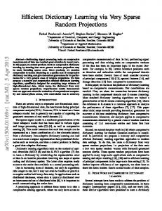


![Very Sparse Random Projections - UCSD CSE [PDF]](https://m.moam.info/img/260x300/very-sparse-random-projections-ucsd-cse-pdf_6479933d098a9e2d128b45e0.jpg)


