Sliding mode control with a robust observer of induction motor

Imene KEBBATI1, Yamna HAMMOU2, Abdellah MANSOURI3, Mohamed BOURAHLA1 Department of Electrotechnical Engineering, U.S.T.Oran, Algeria(1), Department of Maritime Engineering, U.S.T.Oran, Algeria(2), Department of Electrical Engineering, E.N.S.E.T.Oran, Algeria(3),

Sliding mode control with a robust observer of induction motor Abstract. The purpose of this paper is to associate a sliding mode control (SMC) with a powerful nonlinear observer robust flux for an induction motor. We implement this design strategy through an extension of a special class of nonlinear multivariable systems satisfying some regularity assumptions. We show by an extensive study that this purpose is completely satisfactory at low and nominal speeds and it is not sensitive to disturbances and parametric errors. It is robust to changes in load torque, rotational speed and rotor resistance. Streszczenie. Celem niniejszego artykułu jest skojarzenie sterowania ślizgowego z nieliniowym obserwatorem strumienia odpowiednim dla silników indukcyjnych. Realizujemy tę strategię projektowania poprzez rozszerzenie specjalnej klasy układów nieliniowych wielu zmiennych spełniających pewne założenia prawidłowości. Przedstawiono analizę wykazująca, że ten cel jest spełniony dla niskich prędkości i nominalnym, a system nie jest wrażliwy na zakłócenia i błędy parametryczne. Jest odporny na zmiany momentu obciążenia, prędkości obrotowej i oporu wirnika. (Sterowanie ślizgowe silnikiem indukcyjnym z odpornym oberwatorem)

Keywords: Sliding mode control, induction motor, nonlinear observer, rotor resistance Słowa kluczowe: sterowanie ślizgowe, silnik indukcyjny, nieliniowy obserwator.

Introduction The induction motor constitutes a theoretically challenging control problem since the dynamical system is nonlinear, the electric rotor variables are not measurable, and the physical parameters are most often imprecisely known. The control of the induction motor has attracted much attention in the past few decades. Especially the speed sensorless control of induction motors (IM) has been a popular area due to its low cost and strong robustness [1], The new industrial applications necessitate flux and speed variations having high dynamic performances, good precision in permanent regime, and a high capacity of overload over the whole range of position and speed, and robustness to different perturbations. Thus, the recourse to robust control algorithms is desirable in stabilization and in tracking trajectories [2]. Among nonlinear control strategies, sliding-mode control is one of the effective control methodologies for IM drive control because of its disturbance rejection, strong robustness subject to system parameter variations and uncertainties and particularly its simplicity of practical implementation. Upon these advantages so far, many research notes have been reported for IM drives control or estimation, using sliding-mode technique [3]. The sliding mode control proposed by [2,4-6] decouples completely the model of IM actually it is not required to establish a decoupling by field oriented control (FOC) as is usually done in vector control. So the idea is to combinate a sliding mode controller and high gain observer in order to have a strong robustness [7]. This paper is organized as follows. The oriented model of an induction motor is introduced in section 2. In section 3, a robust observer of IM using the high gain is proposed. The sliding mode theory and the design of the sliding mode controllers are presented in section 4. In section 5, the control of rotor flux and motor speed of IM are presented. Finally, we give some concluding remarks on the proposed controller and/observer of IM, and some simulation results are presented. Mathematical model of induction motor A three-phase induction motor with squirrel cage rotor is considered in the paper. Assuming the three-phase AC voltage is uniformly distributed over the stator windings are balanced and is based on the well-known in two phases. equivalent representation of the motor, the model of

induction motor can be described in the fixed coordinate system (α,β) by a set of the first order nonlinear differential equations [1].

K 1  i s   i s  T  r  p  K  r   L U s r s  i   i  K   p  K   1 U s r r s  s Tr  Ls  M 1  i s   r  p   r (1)  r  Tr Tr    M i  1   p   r  r T s T r r r    Ce  f m    L   Jm Jm Jm pM Ce   r i s   r i s Lr





with

  1

L M2 M ; K  ; Tr  r ; L s Lr  L s Lr Rr

 

Rs R M2  r  L s  L s Lr

Here, rα , rβ – the rotor flux components, Usα, Usβ – the stator voltage components, isα, isβ – are the stator current components, σ is the leakage factor and p – the number of pole pairs. Rs and Rr are stator and rotor resistances, Ls and Lr denote stator and rotor inductances, whereas M is the mutual inductance. Ce is the electromagnetic torque, τL is the load torque, Jm is the moment of inertia of the IM, Ω is the mechanical speed, fm is the damping coefficient, Tr is the rotoric time-constant. Nonlinear observer of induction motor The proposed observer uses the measurements of the stator voltage and current, and the rotor speed. More precisely, the observer is designed up to an injection of the speed measurements so that only electrical equations are considered. Consequently, the gain can be updated directly, as described in the theorem, without making use of any kind of transformation. The model is described by:

PRZEGLĄD ELEKTROTECHNICZNY (Electrical Review), ISSN 0033-2097, R. 88 NR 1b/2012

193

 z  F () z  G (u , , z )  y  C z

(2) where

is   r  z1    , z 2   , is   r  is  U s  , y , s u  is  U s   K  Kp  T  i s  U s   , g1 (u , , z1 )   F1 ()   r  K   Kp   i s  U s   Tr  1  M  T is  T  r  p r  r  and g 2 (u , , z )   r  M i  1   p  r   Tr s Tr r  Assume that the system (2) satisfies Assumption’s [8] Then there exists  > 0 such that the System

z  F ( ) zˆ  G (u , , zˆ )  1 ( ) S1C T Czˆ  y 

(3)

Where

I  ( )   2 0

0  2 I  , S1C T   2 2   F1 ()  I 2 

The choice of  permits the pole placement of the motor and the observer according to the speed Sliding mode control The sliding mode technique is developed to solve the disadvantage of other design of non linear control systems. This technique adjust feedback by previously defining a surface, so that the system which is controlled will be forced to that surface, then the behaviour of the system slides to the desired equilibrium point. The main feature of this control is that we only need to drive the error to a switching surface .When the system is in the sliding mode, the system behaviour is not affected by any modelling uncertainties and/or disturbances. Calculation of control laws: The control function will satisfy reaching conditions in the following form: (4)

u  u e  ui

here u is the control vector, ue is the equivalent control vector, it can be interpreted as the average value swing , aside from, it is calculate : S(X)=0 →S(X)=0 , ui is the correction factor and must be calculated so that the stability conditions for the selected control are satisfied.

where



pM ; J m Lr

f 1  i s  r  i s  r ;

f 2  i s  r  i s  r ; k1 , k 2  0  ref and  ref are the time derivative of φref and Ωref, respectively; along

S  0 we have :



(6)



L   f 2  J   k1    ref   ref m 2   Mf1      k 2    ref   ref  Tr





Knowing that

L     is  r  is  r  J m    2 M i  i    s r  s  r Tr 



(7)



 

 

We obtain (8)

 

 

 

d  dt    ref  k1    ref d     ref   k 2    ref  dt

 

Consequently on S ≡ 0 the rotor speed and the square of rotor flux must converge to their references. However from following their reference, it is sufficient to make the sliding surface attractive and invariant. We consider the following proposition: Proposition: We consider the slid surface S=[S1 S2]T defined in (4) and control law sliding mode u  u e  u i

(9)

 0   sign( S1 )  1 u 01 u i   D      0 u 02   sign( S 2 )  u   D 1  A  B  e  

(10)

u 01  A  u 02  B

where

   r D  M r

 r  1 with   M r  Ls

and

    1    f 2  k1 L  p f1  K   A   k1  J m Tr     k 1    1  ref   ref    ui  k signS (X )  (11)  Tr    Tr T k   B   r 2  1   ref  k2 Speed and flux sliding mode controller ref  2 2 2    The objective of SMC is designed for converge the  modulus of the rotor flux vector (ø), and speed (Ω) to their  M 2  1  K  2   reference value øref and Ωref, respectively. For that it is     f1       M i i p f s s   2   T T T proposed that all states are measured, our objective is to r r r      T build a control law u=[ua ub] to force the states that are flux Proof and speed to meet the slide surface S=[S1 S2]T which is 1 Let consider the Lyapunov function V  S T S , so its defined by: 2  ref  L k1 T    S1     ref   f 2  time derivative V  S S



(5)

194



  Jm  T Tr S  r k     2 2 ref  M f1     ref 2 2 






 A B

S 2 

follows:

0   A u S      01  sign( S )  B   0 u 02  The variety S is attractive if: S T S  0 (12)

u 01  A  u 02  B

We can choose u01 u02 such that

 L max  u 01  A  k1  J m (14)   L max u 02  B  k 2   Jm Where  L max  max( L )

0.35 Rr nominal 120% Rr 150% Rr 180% Rr

0.3 0.25

Then the condition of existence of sliding requires only to knowledge the maximum value of torque that the machine and support. However S=0 is invariant if S  0 ; that is to say:

0.2 0.15 0.1

 A u e   D 1   B

0.05

In the design of the control, we assume that all state was measured. Since is only measures the current and the speed are a variable, we will need to estimate a rotor flux for a real time application. Results and simulations Simulation blocks diagrams As a first step, a Simulink/Matlab simulation was realized in order to simulate a motor model according with the proposed observer. The parameters of the motor model are given in the Table 1 [8]. The trajectories of the references speed, flux and load torque are given in Fig. 1. This benchmark shows that the load torque appears at the nominal speed. In spite of a varying speed, the resistive torque is zero. The desired flux remains constant in the asynchronous machine to satisfy the objectives of the fieldoriented control.

0

0

0.02

0.04 0.06 Times (s)

Rr nominal 120% Rr 150% Rr 180% Rr

0.3 0.25 0.2 0.15 0.1 0.05 0 -0.05

0

0.02

0.04 0.06 Times (s)

Speed (rad/s) Flux (Wb)

0.08

0.1

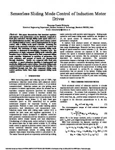
Fig. 3. Observation errors of the flux at a nominal speed of 1500 rpm

0

0

1

2

3

4

5

6

7

8

9

200

1.5 1

150

0.5 0

100 0

1

2

3

4

5

6

7

8

9

Speed (rad/s)

20 Torque (Nm)

0.1

0.35

200

-200

0.08

Fig. 2. Observation errors of the flux at a low speed of 230 rpm

Flux error (Wb)

(15)

0.4718 H 0.0293 kg/m² 2 0.0038 Nm.sec/rad 1.1 KW 220 V 2.6 A 1410 rpm

Lr Jm p fm Pmec Vsn Tsn Ωsn

Study of the nonlinear observer in an open loop First we test the nonlinear observer are open loop (θ = 500) at low and high speed while varying the rotor resistance up to 180%. In the figure 2 and 3, we noted that the estimated flux and the real flux are fully in line after 0.02sec.

Then (13)

Rotor inductance Rotor inertia Pole pair Viscous friction coefficient Mechanical power Nominal voltage Nominal current Nominal speed

Flux error (Wb)

 S 

with S   1      D ui , we can be rewritten S as 

0 -20

0

1

2

3

4 5 Times (s)

6

7

Fig. 1. References trajectories Table 1: Inductor motor parameters Parameter Notation Value Rotor resistance 4.3047 Ω Rr Stator resistance 9.65 Ω Rs Mutual inductance 0.4475 H M Stator inductance 0.4718 H Ls

8

9

50 0 -50 -100 -150 -200

0

1

2

3

4 5 times (s)

6

7

8

9

Fig. 4. Real speed and its reference with Rr variable


195

Sliding mode control SMC In this section (Figure 4-7), the flux is considered measurable and the non-linear control SMC, when analyzing the variation of rotor resistance up to 180% and it also assumes that the torque is zero. we can clearly distinguish that this variation does not affect the controller because the error has not exceeded 0.07rad/s (Fig.5).

Low speed

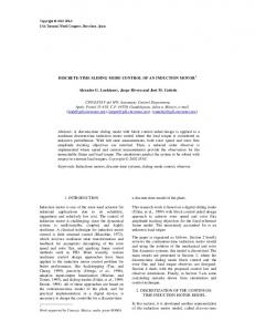
At a low speed of 230 rpm, there is an optimum speed error and flux not exceeding, respectively, 35 rad/s and 4.5 Wb and it vanishes very quickly to 0.03 sec (Fig 8 and 9). 35

0.08

25 Speed error(rad/s)

Rr nominal 150% Rr 180% Rr

0.06 0.04 Error speed (rad/s)

Rr nominal 120% Rr 150% Rr 180% Rr

30

0.02

20 15 10

0 -0.02

5

-0.04

0

0

0.01

0.02 0.03 Times (s)

-0.06

0.04

0.05

Fig. 8. Comparison of error speed for 180% variation in Rr -0.08

0

1

2

3

4 5 times (s)

6

7

8

9

5

Fig. 5. Comparison of the error speed for 180% variation Rr

Rr nominal 150% Rr 180% Rr

4

5 Rr nominal 150% Rr 180% Rr

3 Error flux (Wb)

4

Error flux (Wb)

3

2

1 2 0 1 -1 0

0

0.02

0.04 0.06 Times (s)

0.08

0.1

Fig. 9. Comparison of error flux for 180% variation in Rr 230 rpm -1

0

0.02

0.04 0.06 Times (s)

0.08

0.1

Fig. 6. Comparison of the error flux for 180% variation Rr 6 Reference flux Rr nominal 150% Rr 180% Rr

5

Normed flux

4

Nominal speed

By applying the reference trajectory (Fig. 1) with a load torque zero on interval 0 sec to 1.5 sec, which rises abruptly to 20 Nm stabilized until 2.5sec and then it drops to zero at -20 Nm no 6 s for 1 s, we note that the effect of the load torque is negligible on the speed and flow control. The influence of rotor resistance appears only when the torque is important. As a result the nonlinear controller SMC can be considered robust (Fig.10-13).

3

200 Reference Flux Rr nominal 150% Rr 200% Rr

150

2

100

0

0

0.02

0.04 0.06 times (s)

0.08

0.1

Fig. 7. Real flux and its reference with Rr variable

Performance SMC associated with the nonlinear observer A periodic trapezoidal reference speed is used here to study the tracking performance of the drive system. It is shown in Fig.1, the speed is increased linearly from 0 at t = 1 sec to 150 rad/sec at t = 3.5sec, and decreased linearly to -150 rad/sec at t=5.5sec. Then, the speed is kept constant at -150 rad/sec till t = 8 sec and increased linearly to zero at t = 9 sec. The same trajectory is used to study the performance of sliding mode controller with variation of rotor resistance at 180%

196

Speed (rad/s)

1 50 0 -50 -100 -150 -200

0

1

2

3

4 5 Times (s)

6

7

8

9

Fig. 10. Real speed and its reference


required to obtain the convergence of the observation at low speeds. The efficiency of the control-observer structure has been successfully verified by simulation. The proposed sliding mode control with nonlinear observer demonstrated very good performance, especially; it is robust under rotor resistance variation, external load disturbances and speed tracking. Future work is oriented at experimental validation, including stator time-constant estimation.

25 Rr nominal 150% Rr 200% Rr

20 15

Speed error (rad/s)

10 5 0 -5 -10

REFERENCES

-15

[1] Tian-Jun F.and Wen-Fang X. (2005) “A novel sliding-mode control of induction motor using space vector modulation technique”, ISA Transactions, Vol 44 pp 481–490 [2] Abid M., Mansouri A., Aissaoui A.G., Belabbes B. (2008), “Sliding mode application in position control of an induction machine” Journal of Engineering Vol 59 N°06 pp 322-327 [3] Hajian M., Arab Markadeh G.R, Soltani J. and S. Hoseinnia (2009) “Energy optimized sliding-mode control of sensorless induction motor drives”, Energy Conversion and Management, Vol 50 pp 2296–2306 [4] Abid M., Ramdani Y., Meroufel A.K. (2006), “Speed sliding mode control of sensorless induction machine” Journal Electrical Engineering Vol 57 N°01 pp 47-51. [5] Yazdanpanah R., Soltani J., Arab Markadeh G.R. (2008), “Nonlinear torque and stator flux controller for induction motor drive based on adaptive input-output feedback linearization and sliding mode control” .Energy conversion and management Vol49 pp 541-550. [6] Oliveira J.B., Araujo A.D, Dias S.M., (2010) “Controlling te speed of a three-phase introduction motor using a simplified indirect adaptive sliding mode sheme.” Control Engineering Patrice Vol 18 pp 557-584 [7] Mezouar A., Fellah M.K. and Hadjeri S. (2007) “Adaptive sliding mode observer for induction motor using two-time-scale approach”, Electric Power Systems Research, Vol 77 pp 604– 618 [8] Mansouri A., Chenafa M ., Bouhenna A. And Etien E. (2004) “Powerful nonlinear observer associated with field-oriented control of an induction motor” Int. J. Appl. Math. Comput. Sci., Vol. 14, No. 2, 209–220 [9] Mansouri A. “Contribution à la commande des systèmes non linéaires (Application aux robot et au moteur asynchrone)” (2004) thèse de doctorat. [10] Bouhenna A., Mansouri A., Chenafa M., Belaidi A.(2008), “Feedback Gain Design Method for the Full-Order Flux Observer in Sensorless Control of Induction Motor” International Journal of Computers, Communications & Control, Volume III (2008) N°2 pp. 135-148. [11] Castillo-Toledo B. (2008) “Discrete time sliding mode control with application to induction motors” Automatica vol 44 pp 3036-3045. [12] Inanc N. (2002) “A new sliding mode flux and current observer for direct field oriented induction motor drives”; Elecric power systems research, Vol 63 pp 113-118. [13] Utkin V.I. (1993) “Sliding mode control design principles”, IEEE, Transactions on Industrial Electronics. Vol 40 pp 23-36

-20 -25

0

1

2

3

4 5 Times (s)

6

7

8

9

Fig. 11. Comparison of error speed for 200% variation in Rr Reference Flux Rr nominal 150% Rr 200% Rr

1.15 1.1

Flux (Wb)

1.05 1 0.95 0.9 0.85 0.8 0.75 0.7

0

1

2

3

4 5 Times (s)

6

7

8

9

Fig. 12. Zoom on actual and reference flux 20 Rr nominal 150% Rr 200% Rr

18 16

Current Norm (A)

14 12 10 8 6 4 2 0

0

1

2

3

4 5 Times (s)

6

7

8

9

Fig. 13. Currents norm stator

Conclusion The robust nonlinear observer of a special class associated with SMC for induction motor has been presented. The rotor flux observer accuracy is guaranteed through the stator currents observer, based on the Lyapunov stability theory. The results show that this nonlinear observer offers better performances while tracking the torque, speed and estimating the flux. A major advantage of the method is that very little tuning was

Authors: Miss Imen Kebbati Department of Electrotechnical Engineering, U.S.T.Oran, Algeria. E-mail: [email protected]; Miss Department of Maritime Engineering U.S.T.Oran, Algeria, Email: [email protected]; Prof Abdallah Mensouri Department of Electrical Engineering, E.N.S.E.T.Oran, Algeria. E-mail: [email protected] ; Prof Mohamed bourahla Department of Electrotechnical Engineering, U.S.T.Oran, Algeria. E-mail: [email protected].


197