Sliding Modes in Motion Control Systems

ISSN 0005–1144 ATKAAF 46(1–2), 17–27 (2005) Asif [abanovi}, Nadira [abanovi}, G aĆdać Onal

Sliding Modes in Motion Control Systems UDK 681.511.4 IFAC 5.9.3 Original scientific paper In this paper we discuss the realization of motion control systems in the sliding mode control (SMC) framework. Any motion control system design should take into account the unconstrained motion (generally perceived as a trajectory tracking) and motion of the system in contact with unknown environment (perceived as force control and/or compliance control.) In the SMC framework control is selected to enforce certain preselected dependence among system coordinates, what is interpreted as forcing the system state to stay in selected manifold in state space. In this paper it has been shown that such a formulation allows a unified treatment of the both unconstrained and constrained motion control and, due to the Lyapunov based design, it guaranty the stability of the motion. Moreover control design in this framework allows extension of the solution to control design in interconnected dynamical systems (like mobile robots or bilateral systems). Key words: motion control, sliding mode, hybrid control, nonlinear control, interconnected systems

1

INTRODUCTION

The most salient feature of the Sliding Mode Control (SMC) is the possibility to constrain a system motion in selected manifold in the state space. Such motion in general results in a system performance that includes disturbance rejection and robustness to parameter variations [1]. Restriction of a system motion in a selected manifold, e.g. enforcing sliding mode, forces system states to satisfy selected algebraic constraint, thus reducing order of the system's motion. The development of SMC has gone through oscillations with both very enthusiastic claims and the skepticism regarding the achieved results. In some cases researchers contributed to the confusion, especially in the case of so-called chattering phenomena, through incomplete analysis and design fixes [2, 3, 4, 5]. The complexity and nonlinear dynamics of motion control systems along with high-performance operation require complex, often nonlinear control system design, to fully exploit system capabilities. Basic goal for motion control systems is to achieve smooth stable motion in the presence of unstructured environment, which may consists of another systems being in motion or stationary, with which plant under control can be in interaction (actual or virtual). The contact among systems is resulting in the appearance of the interaction force that should be controlled at the certain level or at least limited to avoid damage. As well known, the mathematical model of motion system with and without contact

AUTOMATIKA 46(2005) 1–2, 17–27

with environment is different and that requires different controllers in order to ensure desired behavior of the system in both cases. In robotics related publications the solution is found in socalled hybrid position/force framework [6], which has been as a concept widely used with numerous modifications [6]. Apparent impedance control [7] is another approach that can ensure the predicted behavior of the system in contact with environment, which in the same way as hybrid control appears in literature with many modifications [7]. In both framework the transient from position control to force/impedance control may cause problems related to oscillation and may lead to instability. Both frameworks when combined with acceleration controller may provide very good behavior of the system. In this paper we will demonstrate a generalized framework for sliding mode approach in the fully actuated mechanical motion control systems with or without interaction with environment. Due to the fact that sliding mode represents a framework for acceleration control [8] implementation the solution we will discuss thus offers all advantages of the acceleration control, like robustness to the parameters uncertainties, the robustness to external disturbances and unique feature of the SMC design the enforcement of desired algebraic constraint among system coordinates. We will demonstrate that hybrid position/force control scheme and the impedance control scheme can be unified and treated in the same way while avoiding the structural change of the controller and thus guarantying sta-

17

Sliding Modes in Motion Control Systems

A. [abanovi}, Nadira [abanovi}, G. Onal

ble behavior of the system. It will be shown that this framework can be naturally extended to control of mechanical systems in interaction. This new framework may be useful in designing bilateral systems or in mobile robotics. The paper is organized as follows. In section 2 the basic results of SMC and design of position and force control for motion control systems in SMC are discussed, in section 3 the new SMC based algorithm that realizes the hybrid position/ force and impedance control is presented, in section 4 the extension of the results obtained in section 3 to bilateral control and mobile robotics will be discussed and in section 5 simulation and experimental results will be shown. 2 SLIDING MODES IN MOTION CONTROL SYSTEMS

So-called sliding mode motion is represented by the state trajectories being forced to stay in the selected state space manifold (sliding mode manifold) with finite time convergence to it. In the continuous time the control that guaranties above properties happens to be discontinuous with high frequency switching, while in the discrete-time the control that guaranty the motion in sliding mode manifold is continuous in the sense of discrete-time systems [9–14]. 2.1 Mathematical Formulation of Control Plant

For »fully actuated« mechanical system (number of actuators equal to the number of the primary masses) mathematical model may be found in the following form M (q )q&& + N (q ,q& ) =F −F e (q ,q& q, e, q & e )   C (q , q& )q& +G (q ,q& ) =N (q ,q& )   d ( t ) = −N (q ,q& ) −F e (q ,q& ,q e ,q& e ) 

(1)

where q ∈ ℜ n stands for vector of generalized positions, q& ∈ ℜ n stands for vector of generalized velocities, q e ∈ ℜ n stands for vector of generalized positions of environment (obstacle), q& e ∈ ℜ n stands for vector of generalized velocities of environment (obstacle), M (q ) ∈ ℜ nxn is generalized positive definite inertia matrix with bounded parameters hence M − ≤ M (q ) ≤ M + , N (q , q& , t ) ∈ ℜ nx1 represent vector of coupling forces including gravity and friction and is bounded by N (q , q& , t ) ≤ N + , F ∈ ℜ nx 1 with F ≤ F0 is vector of generalized input forces and the external forces Fe ∈ ℜ nx1 and d ( t ) ∈ ℜ nx1 stands for the system disturbance. It should be noted that external force, being a result of the system (1) contact with environment or another system thus depending on the generalized coordinates of both sy18

stems Fe = F e (q , q&, q e ,q& e ) ∈ ℜ nx1 . M −, M +, N + and F0 are known scalars. In system (1) vectors Fe ∈ ℜ nx1 and N (q , q& , t ) ∈ ℜ nx1 satisfy matching conditions [12]. External force is a result of the system's interaction with environment and as such depends on the coordinates of both the system and the environment and it can be interpreted as an interaction force. In this framework the environment can be presented by another mechanical system in motion or can be a virtual force perceived to act between systems (like between mobile robots) and not necessarily by a stationary obstacle. Such an interpretation will allow us to formulate approach that encompasses all such problems in one framework. 2.2 Control Problem Formulation

Vector of generalized positions and generalized velocities ζT = ( q , q& ) defines configuration of a mechanical system [13, 14]. Generally the control tasks for system (1) can be formulated as a selection of the generalized force input, which would force system to execute a desired motion in task space. In robotics, desired motion is usually specified as position tracking, control of force resulting from an interaction of system with environment or as a problem obtaining desired apparent impedance of the mechanical system against external force acting on it due to an interaction with environment (system having desired mass-spring-damper dynamics against external force). In the framework of mobile robots the desired task may be specified as a requirement to move without collision or if more robots are present to form certain configuration represented by virtual forces maintained between robots. In order to apply sliding mode framework these control tasks should be defined in the form of a requirement to enforce motion such that configuration of mechanical system ζT = ( q , q& ) tracks desired r r reference configuration ζ r = ( q r , q& r ) , where ( q , q& ) stands for reference generalized position and velocity respectively. This formulation can be expressed in the form in which vector quantity σ = (ζ, ζ r ) is forced to have zero value. This can be interpreted as enforcement of some functional relation σ = (ζ, ζ r ) = 0 nx 1 between generalized coordinates of the system. In general σ = (ζ, ζ r ) = 0 nx 1 can be either linear or nonlinear function of the system's generalized coordinates and time dependent reference configuration such that by enforcing σ = (ζ, ζ r ) = 0 nx 1 the reference configuration is reached and maintained under control. Due to the fact that system configuration ζ cannot be discontinuous σ = (ζ, ζ r ) should be also selected as a continuous function and consequently the reference configuration should be continuous function of time as well. Without loss of generality, in this paper we will assume that function σ = (ζ, ζ r ) is linear combination of geneAUTOMATIKA 46(2005) 1–2, 17–27

Sliding Modes in Motion Control Systems

A. [abanovi}, Nadira [abanovi}, G. Onal

ralized coordinates and their references, as depicted in (2). This format is used in most of the literature related to SMC control of mechanical systems, but as we will demonstrate later in the paper selection of σ = (ζ, ζ r ) as nonlinear function is also acceptable and may lead to very interesting control configurations for system (1).    T σ( ζ, ζ r ) ∈ ℜ nx 1 , G , H > 0,σ = [σ 1 , σ 2 ,...., σ n ]  (2)  G 0   Λ=   0 H  

σ( ζ, ζ ) = G q + H q& − ζ r ( t) = Λζ −ζ r =0 , r

where ζ r ( t ) ∈ ℜ nx 1 stands for the reference configuration of the system and is assumed to be known bounded continuous function with bounded elements and their first order time derivatives, Λ is appropriate composition of matrices G and H. In the sliding mode framework requirement (2) is equivalent to enforcing sliding mode in manifold (3)

{ = {( q , q& ) : G q + H q& − ζ

Sq

r

}

  . r = σ (ζ, ζ ) =0  

Sq = ζ : Λζ − ζ r = σ (ζ ,ζ r ) =0

}

(3)

It is easy to determine the projection of the motion of system (1) into manifold (3) in the following form σ& ( ζ, ζ r ) = Λζ& − ζ& r . Selecting G , H ∈ ℜ nxn as diagonal, the elements of vector function σ = (ζ, ζ r ) are independent and projection of the system's motion in manifold (3) can be represented by ra set of dσi ζ ( t) n first order equations = g i q& i + hi q&&i − i , i = dt dt = 1,2,..,n. The particular solution will then depend on the selection of vector function ζ r ( t ) ∈ ℜ nx 1 thus it can be modified by reference vector ζ r ( t ) ∈ ℜ nx 1 .

  d ζ r ( t)  M q&& = M H −1  −G q&  =M q&& des ,   dt      r   des −1  d ζ ( t ) && q =H  −G q&    dt    

(4)

Which, after some manipulations may be written as     . d  −1  d ζ r ( t ) = H  −G q    d t   dt  

&& q = q&& des , && q des

(5)

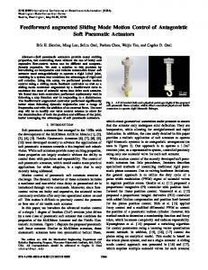
The sliding mode motion (5) in manifold (3) for fully actuated mechanical system (1) depends only on the selection of the manifold (matrices G, H) and the reference configuration of the system ζ r ( t ) ∈ ℜ nx 1 . The sliding mode motion in sliding mode in manifold (3) is equivalent to the acceleration control [8] with desired acceleration being expressed as in (5). After initial transient, defined by the matrices G and H, the steady state solution is determined by the selection of the reference configuration. By selecting reference configuration ζ r ( t ) one can expect to be able to attain different control tasks. Motion in sliding mode is robust against the plant parameter changes and the generalized disturbance vector d ( t ) = −H [N ( ζ) +F e (ζ, ζ e ) ] as long as actual control resources satisfy condition Feq ≤ F0 . The structure of the sliding mode control system is depicted in Figure 1.

2.3 Equations of motion in sliding mode

If sliding mode is enforced in manifold (3) then equivalent control, being solution of σ& F = F = G q& + H q&& − eq

dζ r ( t ) dt

=0 , F = Feq

under the assumption that G , H ∈ ℜ nxn are constant and H−1 exists, is determined as  dζ r ( t )  Feq = M H −1  G q&  +N ( ζ ) +F e (ζ, ζ e ) −  dt   

and the equations of motion for system (1) with sliding mode in manifold (3) can be derived in the form AUTOMATIKA 46(2005) 1–2, 17–27

Fig. 1 (a) The structure of the SMC motion control system and (b) the structure of equivalent closed loop system (5)

In sliding mode on manifold (3) system (1) realizes an acceleration controller with desired acceleration being q& des = d (H −1 ( ζ r ( t) −G q )) . This indicates dt that results attained in acceleration control framework may be realized in sliding mode framework as well. In the sliding mode framework desired configuration of the system can be realized while all advantages of the acceleration control framework can be retained. The fact that the closed loop sys19

Sliding Modes in Motion Control Systems

tem motion (5) is the same as the equation of sliding mode manifold is due to the specifics of fully actuated mechanical system's dynamics (1). In order to complete design the selection of the control input and the selection of the reference configuration for different tasks should be discussed. 2.4 Selection of control input

Design of control inputs for system (1), (2) with sliding mode in manifold (3) may follow different approaches. All approaches have common requirement to derive the control input such that the stability of the solution σ( ζ, ζ r ) = 0 nx1 is enforced. This could be satisfied if one can derive a control input which guaranty that Lyapunov stability conditions are satisfied. Since control system requirements are met if σ( ζ, ζ r ) = 0 nx1 is stable solution for system (1) a Lyapunov function candidate may be selected as as v = 1 σT σ with its first time derivative being 2 v& = σT σ& . To ensure stability the Lyapunov function derivative is required to be negative semi-definite and v(0) = v&(0) = 0 . This can be guarantied if derivative of Lyapunov function has specific form so to ensure that v& = σT σ& = −σ T Ψ (σ) < 0 . Then one can derive σT (σ& + Ψ (σ) )

σ ≠0

σ ≠0

= 0 and consequently con-

trol should be selected to satisfy σ& + Ψ (σ ) = 0 ⇒ F = F eq − M H −1Ψ (σ ).

Obviously the structure of control will depend on σ), which should the selection of vector function Ψ(σ be selected such that σ& + Ψ (σ ) σ ≠ 0 guaranties that solution σ = 0 is reached in finite time. In literature this function is most often selected as Ψ ( σ ) = = M o sign( σ ) and the resulting control is discontinuous F = − F0 sign( σ ) ⇒F i = − F0 i sign( σ i ) , i = 1,..., n Feq ≤ F0 [13]. Such a control is simple but in mechanical systems may be hard to realize due to the fact that forces are continuous function, and in addition to that discontinuous control may excite high frequency dynamical terms thus causing chattering. In literature on SMC [14] many different solutions are proposed to deal with this problem. In the following paragraph a solution suitable for application in discrete-time systems will be discussed.

A. [abanovi}, Nadira [abanovi}, G. Onal

1 F (kT + T ) = sat (F eq ( kT ) −M H −D σ( kT )),

D>0

(6)

where sat(•) stands for saturation function with bounds being ± F0. Control (6) is continuous (in a sense that due to ζ,ζ ζ r) = 0nx1 is continuous its interthe fact that σ(ζ -sampling change is o(T) order) but it still requires information on systems parameters and external disturbances for calculation of equivalent control  d ζ r (t)  Feq = M H −1  −G q&  +N +F  dt   

ext .

It has been shown in [15] that by applying sample and hold process with sampling interval T, the discrete-time realization of control (6) can be approximated as depicted in (7) F ( k + 1) = sat (F ( k ) + −1

+ M H T −1 ((1 −D T ) σ( k ) − σ ( k − 1))),

(7)

Implementation of algorithm (7) requires information on distance from sliding mode manifold and inertia matrix. Application of control (7) to system (1), (3) leads to the σT ( k )σ ( k − 1) = σ T ( k )( I − TD )σ ( k).

(8)

In [10] and [15] it is proven that for diagonal matrix D and T D ≤ I (8) presents necessary and sufficient condition for existence of sliding mode in manifold (3) for system (1) and that reaching phase takes finite time. Since (7) is an approximation of (6) the error introduced by this approximation can be determined as σ& ( k ) + Dσ ( k ) = (d ( k ) −d ( k −1))T   d ( t ) = −H [N ( ζ) +F e ( ζ, ζ e ) ] 

(9)

This shows that the motion of the system has an error of the o(T 2) order under the assumption that the disturbance d(t) is continuous. 3 THE GENERALIZATION OF SMC IN MOTION CONTROL

2.5 Discrete-time sliding mode control

3.1 Modification of System Configuration in SMC

It had been shown that in discrete-time systems sliding mode could be enforced by continuous control input [14]. Below one way of achieving such control in system (1) is based on enforcing sliding mode in manifold (3) by selecting Ψ ( σ ) = Dσ ; D > 0 so that the discrete-time control, with sampling in terval T, can be expressed as

By changing vector function ζr(t), which plays a role of the reference configuration in (5), the system configuration could be modified so that system specifications are met. This offers a possibility to solve different control problems by adopting different structure of the reference configuration ζr(t). Since trajectory tracking is one of the tasks in ro-

20

AUTOMATIKA 46(2005) 1–2, 17–27

Sliding Modes in Motion Control Systems

A. [abanovi}, Nadira [abanovi}, G. Onal

botic systems it will be natural to assume that function ζr(t) depends on the desired trajectory of the system. In addition, while in contact with environment, due to the interaction forces motion system is required to modify its trajectory in order to satisfy the safety of the interaction with environment. One possible structure of function ζr(t) that includes both requirements may be selected as follows in (10)  ζ ( t ) = Γσ r + ϕ( t)  σ r = Λζ d ( t ) = G q d + H q& d 

This can be interpreted as if system under control acts as a mass-spring-damper with equivalent mass being Me = H, Equivalent spring Kp = GD and equivalent damper Kd = G + DH as depicted in Figure 2. After reaching sliding mode manifold motion of the system (13) is described by σ = 0 or H (q& − q& d ) +G (q −q d ) = ϕ( t), Γ =I .

(14)

r

(10)

where q d , q& d stands for desired generalized position and velocity respectively, matrices G and H specify the reference trajectory, matrix Γ may modify desired trajectory and vector function ϕ(t) might shift reference trajectory without its modification. By applying control (6) or (7) the motion of the system (1) during reaching phase becomes d ϕ( t )  λ& (ζ, ζ r ) + Dλ (ζ ,ζ r ) = +D ϕ( t)  dt  r  λ ( ζ , ζ ) = Λζ − Γ Λζ = σ q − Γ σ r  σ q = Λζ = H q& + G q

 d d d σ r = Λζ = H q& + G q 

The behavior can be interpreted as a spring-damper system in contact with environment acting with force Fe = ϕ(t) as depicted in Figure 3. Since reaching stage is defined by design parameter D one can shape the overall transients of the system by selecting D. If D is selected large enough the reaching stage is short and the motion of the system is defined by (14).

(11)

(12)

Fig. 3 The interpretation of the SMC closed loop system in contact with environment

what represents second order system transient determined by the design parameters Γ, G, H and D.

In order to illustrate above results, motion of single d.o.f. system defined as in (15) and (16) is simulated

Based on (5), (10) and (11) it is apparent how to derive a unifying framework for control of fully actuated mechanical system (1) in SMC framework. In steady state λ ( q , q r ) = (σ q − Γσ r ) = ϕ( t) thus the actual configuration of system (1) under control (6) will track reference configuration modulated by matrix Γ with offset defined by vector valued function ϕ(t). By selecting Γ = I and ϕ(t) = 0 the trajectory tracking mode is attained. If, on the other hand, Γ = I, ϕ(t) ≠ 0 is selected, trajectory tracking will be achieved with error defined by particular solution of (11) and reaching phase motion (11), (12) defined as q ) + (G + DH )( ∆q& ) +G D ( ∆q ) = d ϕ( t) +D ϕ( t)  ( ∆&& dt  . (13) d  ∆q = q − q

Fig. 2 The interpretation of the SMC in reaching phase

AUTOMATIKA 46(2005) 1–2, 17–27

x& = v   mv& = K t u − Fd 

(15)

  . Fd = 15(1 + 0.5 cos(12.56 t) +0.25 sin(37.68 t)) + 0.5 v + Ffr + Fe 

m = 0.1(1 + 0.25 cos(64.28 t))

K t = 0.64(1 + 0.2 cos(128.28 t))

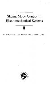
(16) The reference trajectory is selected to be sinusoidal with frequency 1 Hz and amplitude 0.3 m. The controller is selected as u(k + 1) = sat(u(k) + η((1 − dT)σ(k) − σ(k − 1))), with parameters of the controller have been selected d = 100 and η = 120, and sliding mode manifold is determined as σ = C∆ x + ∆ν − ϕ(t) with C = 100 and ϕ(t) = 10 sin(31.4 t). All controller parameters are kept constant for all experiments. In Figure 4 the position x and its reference xr, the reference σr = Cxr + νr and actual value σ = Cx + ν, position error ε(t) = xr − x and force in contact with environment (assumed to be at the position defined by reference xr) are depicted for different values of the parameter ϕ = {−10,10}. 21

Sliding Modes in Motion Control Systems

Fig. 4 The transients for different values of the parameter ϕ(t) = = 10 sin(31.4 t) and σ = (Cx + v) − (Cx ref + vref) − ϕ(t) − αFe in (14)

The contact force is defined by Fe = 1000(x − xr) + + 50(ν − νr). For better presentation force is depicted with gain 0.002. The behavior of the system is as expected. Despite the large changes of the system parameters and disturbance the motion of the system is tracking reference and modulation of the system motion by function ϕ(t) is fully confirmed. In the contact with environment the controlled system reacts as virtual impedance creating a force Fe due to the contact and this force depends on form and value of ϕ(t).

A. [abanovi}, Nadira [abanovi}, G. Onal

Fig. 6 The transients for different values of the parameter ϕ(t) = = 10 sin(31.4 t) − αFe , β = 0.85(1 + 0.25sin(12.56 t)) , α = 0.25 and σ = (Cx + v) − (Cx ref + vref) − ϕ(t) − αFe in (17)

By selecting ϕ(t) = 10 sin(31.4 t) − αFe the motion of the system (15), (16) under the same control as applied in Figure 4 is as depicted in Figure 5. As expected the trajectories of the system in comparison with these presented in Figure 4 are modified during the time when tip is in contact with obstacle. The modification of the system trajectory is due to the interaction force in contact with environment. Finally let us analyze the influence of the parameter Γ on the system behavior. For system (15), (16) the sliding mode manifold is selected in the following form σ = (Cx + v) − β(Cx ref + v ref ) − ϕ( t ) − αFe

(17)

with β = 0.85(1 + 0.25 sin(12.56 t)). The transients under the same control as in Figure 4 and Figure 5 are depicted in Figure 6. The changes in the system trajectory are easy to detect thus showing the possibility to modulate the motion by changing parameter Γ. In order to verify transient behavior of the system in last diagram in Figure 6 the changes in sliding mode manifold are depicted. It can be seen that the controller (6) is forcing the value of sliding mode manifold to stay at zero despite the parameter changes and the changes in manifold parameters. 3.2 General Form of Sliding Mode Manifold Fig. 5 The transients for different values of the parameter α = 0.25, ϕ(t) = 10 sin(31.4t) − αFe and σ = (Cx + v) − (Cx ref + vref) − ϕ(t) − αFe in (17)

22

In order to unify the control tasks for system (1) one should modify (10) in order to include the trajectory tracking, the force control and the compliance. In the previous example we demonstrated AUTOMATIKA 46(2005) 1–2, 17–27

Sliding Modes in Motion Control Systems

A. [abanovi}, Nadira [abanovi}, G. Onal

that by changing matrix Γ and vector ϕ the system motion could be modified. One way of implementing hybrid control framework is to change the position reference whenever system is in contact with environment in such a way that the interaction force is maintained at desired profile. Since in SMC the reference is defined as a desired system configuration σ r ( t ) = ΓΛζ r ( t ) = = Γ (G q r ( t ) + H q& r ( t )) the modification of the system configuration due to the interaction force Fe can be made by making matrix Γ a function of the difference between desired and actual force profile. On the other hand the one can ask for combining the modification of the system trajectory in contact with environment proportional to the force Fe. Taking all in account the modification of the system motion due to the interaction force in SMC framework can be achieved by making reference configuration of the system as in (18) ζ r ( t ) = Γ ( ∆Fe )( G q d + H q& d ) − αF e

(18)

and selecting control to enforce the configuration of the system H q& + G q = σ q to track its reference, or in other word enforcing sliding mode in manifold (19)

{ = {q , q& : σ ( ζ, ζ , ζ

Sq = q , q& : ( Γ( ∆F e )σ r (ζ r ) − σ q (ζ r )) − αF e (ζ ,ζ e ) =0 Sq

e

H q& + G q = σ q ;

r

) =0

}

H q& d +G q

d

=σ r

}

 .    (19)

which contact force should be controlled proportional to force error is a sufficient (but not the best way) of controlling the contact force. In the directions where forces should not be maintained at the required level but either trajectory tracking or compliance control coefficients of matrix Γ(∆Fe) should be kept at 1. The structure of such a controller is depicted in Figure 7.

Fig. 7 The structure of the SMC system that ensures the stability of system (1) in manifold (19) under control (7)

The Sliding mode controller is the same as depicted in (7) and the closed loop transient is described by (11). In the directions in which compliance is maintained the system acts as a damper spring system and the dynamics is defined by ∆q& + C ∆q − αF e =0 . The behavior of the generalized system with a sliding mode manifold (19) and control (7) is simulated for single axis system described by (15) and (16). Parameters of the controller have been selected C = 200 and D = 250 and are kept constant for all experiments. The results are depicted in Figure 8.

Matrix α can be interpreted as a compliance parameter. This matrix is diagonal with elements having nonzero value in the directions in which compliance is to be maintained and having zero value in the directions in which either contact force or trajectory tracking should be maintained. The effectiveness of changing matrix Γ(∆Fe) is demonstrated in the previous example in Figure 6 but a design procedure is yet to be established. In sliding mode in manifold (19) with motion of syΓ(∆Fe)σ σr − σq ) − stem (1) can be represented by (Γ − αFe = 0 what can be rewritten in the following form (20) ( σ r − σ q ) − α Fe − (I − Γ ( ∆F e )) σ r =0 ( σ r − σ q ) = α Fe + (I − Γ ( ∆F e )) σ r .

(20)

Motion (20) can be interpreted as depicted in Figure 3 – a spring damper system in contact with environment that reacts with force (for α = 0) equal σr. By selecting matrix Γ(∆Fe) as to Fe = (I − Γ(∆Fe))σ diagonal with diagonal elements in the directions in AUTOMATIKA 46(2005) 1–2, 17–27

Fig. 8 The trajectory tracking and force control in contact with unknown obstacle and α = 1 in (19). Obstacle defined as xa = 0.1(1 + + 0.3sin(25t)), force in contact with environment is calculated as Fe = 1000(x − xa) + 50(v − va)

23

Sliding Modes in Motion Control Systems

A. [abanovi}, Nadira [abanovi}, G. Onal

The effectiveness of the proposed control is confirmed. The proposed control (7) enforces the existence of sliding mode in manifold (19) and the change of the mode of control (position/force/compliance) is smooth due to the fact that all controls are realized by position controller with constant structure and change of the mode is reflected in the change reference configuration. Another solution of position/force/compliance control in the SMC framework can be devised by putting Γ = I and selecting vector ϕ as a function of force control error as well as the compliance coefficient. The reference configuration of the system can be then defined as in (21) ζ r ( t ) = ( G q d + H q& d ) + β ( ∆F e ) − αF e .

(21)

The sliding mode manifold now has a form as in (22)

{

σ r = G q d + H q& d ;

}

= σ =0  . σ q =G q +H q& 

S = q , q& : σ q − σ r − β ( ∆F e ) + αF

e

(22)

Under control (7) expected behavior of the system should be the same as in the previous case. Indeed simulation of the behavior of the system (15), (16) with control (7) and sliding mode enforced in manifold (21) with the same parameters for references and the controller as in case presented in Figure 8 is depicted in Figure 9. No visible differences in the system behavior are observed as expected from the theoretical analysis.

Fig. 10 The trajectory tracking and force control in bilateral system w/o contact with unknown obstacle force in contact with environment is calculated as Fe = 1000(x − xa) + 50(v − va)

The same framework can be applied for bilateral systems control. To demonstrate it master and slave systems both as defined in (15), (16) are simulated. The slave system is controlled to follow the master system position while not in contact with obstacle and while in contact with obstacle slave is controlled to have certain compliance and/or to limit contact force to certain constant level while master is forced to track slaves position as a reference. Both master and slave are identical and have identical controllers. The behavior is depicted in Figure 10 and it shows that proposed approach may be successfully used in this case too. The same structure may be applied for mobile robots specifying interaction among them by a virtual force that should be controlled. The systems requirements in this case are similar as in previous situation but this is out of the scope of this paper. 3.3 Experimental verification

Experimental verification of the above results is obtained in controlling of a single axis Piezomechanik's PSt150/5/60 stack actuator (xmax = 60 µm, Fmax = 800 N, vmax = 150 Volt) connected to SVR150/3 low-voltage, low-power amplifier. Force measurement is accomplished by a load cell placed against the actuator (Figure 11). The entire setup is connected to DS1103 module hosted in a PC (Figure 12). Fig. 9 The trajectory tracking and force control in contact with unknown obstacle and α = 1 in (21). Obstacle defined as xa = 0.1(1 + + 0.3sin(25t)), force in contact with environment is calculated as Fe = 1000(x − xa) + 50(v − va)

24

In all experiments the parameters of the sliding mode controllers are kept as C = 800, D = 2500. The experiments include the trajectory tracking and a AUTOMATIKA 46(2005) 1–2, 17–27

A. [abanovi}, Nadira [abanovi}, G. Onal

Sliding Modes in Motion Control Systems

Fig. 11 Structure of the Experimental Setup

Fig. 15.a Hybrid controller. Upper graph: tip position its reference and lover graph force and its reference

Fig. 12 Simplified Structure of the Experimental Setup

Fig. 15.b Hybrid controller – transition from force to position tracking

Fig. 13 Tracking of the sinusoidal reference for a PZT actuator. Sliding mode control with disturbance compensation feedback

Fig. 14 Tracking of the sinusoidal reference for a PZT actuator. Sliding mode control with disturbance compensation feedback

AUTOMATIKA 46(2005) 1–2, 17–27

Fig. 15.c Hybrid controller – transition from position to force tracking

25

Sliding Modes in Motion Control Systems

combination of the trajectory tracking and force control in accordance with algorithm (7). The behavior of the sliding mode controller depicted in Figure 13 and sliding mode controller with disturbance observer depicted in Figure 14 are similar but error for the system with disturbance observer is about 50 % smaller. In addition the output noise is much smaller in the system with disturbance observer. This shows the effectiveness of the application of the disturbance observer together with SMC. In Figures 15.a, b and c the experimental transients of hybrid control for PZT actuator with and without contact with unknown obstacle are shown. The capability of tracking both position and force is demonstrated and the smooth transient from force to position and from position to force tracking is shown. The behavior of the system is as theoretically predicted. Very similar situations are depicted in Figure 16 with triangular force reference in order to depict fast transients from one mode of control to another. The smooth transients are observed what confirms validity of the developed approach.

A. [abanovi}, Nadira [abanovi}, G. Onal

and interaction force control can be formulated in the unified way. A general framework for the hybrid control in fully actuated mechanical systems is proposed and its realization in two different forms had been shown and stability has been proven. It has been shown that proposed framework does not require switching between position/force modes and that transient between them is smooth. It also allows natural extension to bilateral systems and control of virtual interaction in mobile robots. Proposed method represents general solution in a sense that allows application for interacting systems with interaction being either actual or virtual force. REFERENCES [1] V. I. Utkin, Sliding Modes in Control and Optimization. Springer-Verlag, 1992. [2] J-J. Slotine, Sliding Mode Controller Design for Nonlinear Systems. Int. J. Control, Vol. 40, No. 2, 1983. [3] W. J. Wang, G. H. Wu, Variable Structure Control Design on Discrete-time Systems – Another Point Viewpoint. Control-theory and advanced technology, Vol. 8, no. 1, pp. 1–16. [4] R. A. DeCarlo, S. H. Zak, G. P. Matthews, Variable Structure Control of Nonlinear Multivariable Systems: A Tutorial. Proc of IEEE, Vol. 76, No. 3, 1988. [5] V. I. Utkin, Sliding Mode Control Design Principles and Applications to Electric Drives. IEEE Tran. Ind. Electr., Vol. 40, No.1, pp. 421–434, 1993. [6] M. R. Raibert, J. J. Craig, Hybrid Position/Force Control of Manipulators. J. Dyn. Sys. Contr., Vol. 102, 126–133, 1981. [7] N. Hogan, Impedance Control: An Approach to Manipulation. J. Dyn. Sys. Meas., Contr., Vol. 107, 1985. [8] K. Ohnishi, Masaaki Shibata, Tushiyuki Murakami, Motion Control for Advanced Mechatronics. Transactions on Mechatronics, IEEE, Vol. 1, No. 1, pp. 56–67, 1996. [9] S. V. Drakunov, V. I. Utkin, On Discrete-time Sliding Modes, Proc. of Nonlinear control system design Conf., March 1989, Capri, Italy, pp. 273–78. [10] K. Furuta, Sliding Mode Control of a Discrete System. System and Control Letters, Vol. 14, no. 2, 1990, pp. 145–52. [11] V. I. Utkin, Sliding Mode Control in Discrete Time and Difference Systems, Variable Structure and Lyapunov Control. Ed. by Zinober A. S., Springer Verlag, London, 1993.

Fig. 16 Hybrid controllers. Upper graph: tip position its reference and lower graph force and its reference

[12] B. Drazenovic, The Invariance Conditions in Variable Structure Systems. Automatica, vol. 5, pp. 287–295, Pergamon Press, 1969.

4 CONCLUSIONS

[13] V. Utkin, J. Guldner, J. Shi, Sliding Modes in Electromechanical Systems. Taylor & Francis, 1999.

In this paper the application of the discrete-time sliding mode control framework in motion control in is discussed. The closed loop system robustness is proven and the equivalency with acceleration control method is established. It has been demonstrated that, due to the robustness property of the systems in sliding mode and selected specific way of defining the reference configuration of mechanical systems, a general solution for position tracking

26

[14] [abanovi}, N. [abanovi}, K. Jezernik, Sliding Modes in Sampled-Data Systems. Automatika, Publisher KoREMA-IFAC, Zagreb, Vol. 44, 3–4, 2003. [15] Seiichiro Katsura, Yuichi Matsumato, Kouhei Ohnishi, Analysis and Experimental Validation of Force Bandwidth for Force Control. International Conference on Industrial Technology, IEEE, pp. 796–801, 2003. [16] Watura Iida, Kouhei Ohnishi, Sensorless Force Control with Force Error Observer. International Conference on Industrial Technology, IEEE, pp. 157–162, 2003.

AUTOMATIKA 46(2005) 1–2, 17–27

A. [abanovi}, Nadira [abanovi}, G. Onal

Sliding Modes in Motion Control Systems

Klizni re`imi u sustavima upravljanja gibanjem. U ovom se ~lanku razmatra realizacija sustava upravljanja gibanjem zasnovana na kliznim re`imima. Pri sintezi bilo kojeg sustava upravljanja gibanjem treba uzeti u obzir neometano gibanje, op}enito tretirano kao slije|enje trajektorije, i gibanje sustava u kontaktu s nepoznatom okolinom, tretirano kao upravljanje silom i/ili upravljanje prianjanjem. Kod upravljanja zasnovanog na kliznim re`imima upravlja~ki se signal odabire tako da odr`ava unaprijed zadanu ovisnost me|u varijablama sustava, tj. sustav se giba po zadanoj hiperravnini u prostoru stanja. U ovom je ~lanku pokazano da takva formulacija problema upravljanja omogu}uje jedinstveno tretiranje i neometanog gibanja i gibanja u kontaktu s okolinom, a zbog sinteze zasnovane na teoriji Ljapunova jam~i se stabilnost gibanja. K tome, sinteza sustava upravljanja zasnovana na predlo`enoj metodologiji mo`e se pro{iriti i na me|uovisne dinami~ke sustave, kao {to su mobilni roboti i bilateralni sustavi. Klju~ne rije~i: sustavi upravljanja gibanjem, klizni re`imi, hibridno upravljanje, nelinearno upravljanje, sustavi s dinami~kim vezama

AUTHORS’ ADDRESSES Asif [abanovi} Nadira [abanovi} Sabanci University, FENS Orhanli-Tuzla, 34956 Istanbul, Turkey @sabanciuniv.edu {asif,nadira}@ G aĆĆdaćć Onal Carnegie Mellon University Pittsborgh, USA @cmu.edu cagdas@ Received: 2005–12–01

AUTOMATIKA 46(2005) 1–2, 17–27

27