Jun 15, 2017 - iments [14, 15], a more basic question remains unan- swered: can the ... from the XXZ spin. arXiv:1706.05026v1 [cond-mat.dis-nn] 15 Jun 2017 ...
Slow Dynamics in Translation-Invariant Quantum Lattice Models ˇ Alexios A. Michailidis,1 Marko Znidariˇ c,2 Mariya Medvedyeva,2, ∗ Dmitry A. Abanin,3 Tomaˇz Prosen,2 and Z. Papi´c1
arXiv:1706.05026v1 [cond-mat.dis-nn] 15 Jun 2017
1
School of Physics and Astronomy, University of Leeds, Leeds, LS2 9JT, United Kingdom 2 Physics Department, Faculty of Mathematics and Physics, University of Ljubljana, 1000 Ljubljana, Slovenia 3 Department of Theoretical Physics, University of Geneva, 24 quai Ernest-Ansermet, 1211 Geneva, Switzerland (Dated: June 19, 2017)
Many-body quantum systems typically display fast dynamics and ballistic spreading of information. An exception are many-body localized systems, where quenched disorder causes the information to spread much slower, i.e., logarithmically in time. Here we address the open problem of how slow the dynamics can be in generic lattice systems with local interactions and no disorder. We identify a class of one-dimensional models where the dynamics is remarkably slow, i.e., the dynamics is indistinguishable from that of localized systems at the time scales and system sizes accessible by matrix-product state simulations. We develop a method based on degenerate perturbation theory that quantitatively captures the long-time dynamics of such systems. Our method allows to classify the types of delocalization processes and paves the way towards a general understanding of slow dynamical regimes in translation-invariant systems in arbitrary dimensions.
Introduction.–One of the central questions of quantum statistical physics is how isolated many-body systems reach thermal equilibrium. The process of thermalization results from the spreading of quantum information into non-local degrees of freedom during the system’s unitary evolution. In ergodic systems, this spreading is fast (ballistic), and the individual eigenstates of the system are effectively thermal states [1–3]. On the other hand, there is growing interest in the non-ergodic systems, which include integrable models [4] and many-body localized (MBL) systems [5–7]. Although these two classes of systems have very different properties, they are believed to share a common characteristic: an extensive set of integrals of motion. In the case of MBL, these are Local Integrals of Motion (LIOMs) [8, 9], which originate from strong disorder and strongly constrain the quantum dynamics in MBL systems, e.g., the spreading of quantum information is very slow (logarithmic) in time [10, 11]. While the existence of MBL phases has been established in disordered 1D models [12, 13] and localized degrees of freedom have been measured in recent experiments [14, 15], a more basic question remains unanswered: can the properties of MBL systems, in particular their slow dynamics, be mimicked by translationinvariant models? Intuitively, one imagines a system described by the Hamiltonian H = H0 + λV , where H0 is a classical potential energy and V is a quantum hopping (tunneling) term. A sufficiently complex H0 might generate a complicated landscape in the Fock space, and possibly localize the system at small but finite λ in the absence of disorder. More generally, this is related to the open question of integrability breaking in quantum systems. Namely, it is not known if the integrability breakdown generically proceeds in a smooth, classical-like KAM style [16], where non-ergodic regions remain for small λ, or if the quantumness instead fosters an immediate restora-
tion of ergodicity at asymptotic time scales. Recent works have sought analogs of MBL in translation-invariant models [17–33]. While some signatures of MBL-like dynamics have been observed [17, 19, 21, 24], the relevance of non-perturbative effects for delocalization has also been pointed out [23]. Moreover, Ref. [22] argued that ergodicity is restored in the thermodynamic limit, resulting in a “quasi-MBL” phase. This is consistent with the observation made in Ref. [34] that the disorder-free systems are prone to finite size effects: when the unperturbed energy E0 � λ, the density of states of a finite system splits into non-overlapping bands. Such a system may exhibit signatures of MBL, but it would not necessarily be representative of the thermodynamic limit. Thus, despite much effort, current understanding of MBL in translation-invariant systems remains less complete than that of disordered systems. In this paper we introduce a broad class of 1D lattice models with local interactions and show they exhibit slow, MBL-like dynamics in the thermodynamic limit. The models contain V , a single-particle hopping term, and H0 , which consists of k ≥ 2-body interactions between particles. In contrast to previous work [19–22], the models studied here include only one particle species, which makes them more amenable to numerical simulations. We develop the analytic description of the longtime dynamics by means of a degenerate perturbation theory (DPT) for the decay of an initial inhomogeneity. While related perturbative arguments have been used for qualitative descriptions of particular models [21, 23], the DPT below is shown to be a general diagnostic of the possible delocalization processes which yields a quantitatively accurate description of the long-time dynamics. As a demonstration, we study a concrete model with k = 3body interactions whose dynamics, in the 1st order DPT, is shown to be strikingly different from the XXZ spin
2 chain. Moreover, we provide strong numerical evidence that this 3-body model displays slow, log-like entanglement growth in large systems (L . 200 particles). Thus, its slow dynamics would practically be indistinguishable from that of an MBL system at the experimentally relevant time scales. At the same time, we show that the 3-body model delocalizes at (much longer) time scales in the 2nd order DPT. These conclusions directly generalize to other types of k-local models, where a slow dynamical regime precedes the ultimate delocalization at a finite time, which can be estimated using the DPT diagnostic. Model with slow dynamics.–Consider the following 1D open chain of spins 21 and length L where H0 = J 1
L−1 X i=1
λV =
λ 2
L−1 X
3 σi3 σi+1 + J2
L−2 X
3 σi3 σi+2 + J3
i=1
− + (σi+ σi+1 + σi− σi+1 ),
L−2 X
3 3 σi3 σi+1 σi+2 ,
0.34*log2(t)-0.8
ladder
t=10
S(j) z(j) S(j)
t=10
S(j) z(j)
j
S(j)
j
i=1
(1)
i=1
{σjα } is the Pauli basis on site j and σj± = (σj1 ± iσj2 )/2. Interaction amplitudes Jk are taken to be of the same order, J, and irrational to avoid commensurate terms in the DPT demonstrations we choose √ below. For √ numerical √ J1 = 2/4, J2 = 3/4, J3 = 5/8, but our results are not sensitive to these precise values. We are interested in the dynamics for weak breaking of integrability, λ � J, and we first consider entanglement entropy. Entanglement entropy on a bipartition A ∪ B of the system is defined as S = −trA ρA log ρA , where the reduced density matrix ρA = trB |ψi hψ| is obtained by tracing out the degrees of freedom of B. We perform a global quench from �the product state N � θ θ |ψi = j cos 2j |↓j i + eiϕj sin 2j |↑j i . Here ϕj is a uniform random phase, while θj is obtained from a random uniform variable ξj ∈ [−1, 1] by cosr θj = ξj . Parameter r biases the orientation of each spin on the Bloch sphere. Our results are independent of the choice of r [35] and we fix r = 11 for optimal balance between state-to-state fluctuations and the magnitude of S, allowing for longest simulation times. In Fig. 1(a) we show the representative dynamics of S in the model (1) starting from a single product state. Time evolution is carried out using time-evolving blockdecimation (TEBD) algorithm [36]. We consider a large chain of L = 64 sites, set λ = 0.2, and use bond dimensions up to 350. On the time scales t . 200, we observe a clear difference between the 3-body model (1) (red) and XXZ model (J2 = J3 = 0) (blue). In the XXZ case, S ∝ t, while in the 3-body case the data is consistent with S(t) ∝ log t [35]. Phenomenologically, the linear growth of entropy in the XXZ model is due to the propagation of coherent quasiparticles with velocity ∼ λ [37, 38]. Reducing the hopping only affects the slope S(t) ∝ c(λ)t, where c(λ) ∝ λ, and the XXZ chain remains delocalized for arbitrarily small λ. Tiny deviation from linear growth
S(j)
t=50
S(j) z(j) j
Figure 1. (Color online.) (a) Slow dynamics of entanglement entropy (averaged over all cuts) for the model in Eq. (1). Entropy growth can be fit with a logarithmic function of time, in contrast to the linear growth in the XXZ model (blue). Inset shows the magnetization profile of the initial state. (b) Snapshots of entropy S(j) at the bond j, j + 1 and magnetization hσj3 i at times denoted by red dots in (a). A blocking region (shaded) does not decay on the given time scale and suppresses the growth of entropy. (c) Same as (b) but for the XXZ model, where the blocking region decays by t ∼ 50. In all simulations, L = 64, and λ = 0.2.
in the XXZ model is likely due to finite L = 64 [35]. In contrast, the spreading of entropy in the 3-body model for small λ appears logarithmic, even in a very large system, which is reminiscent of MBL physics. To understand the mechanism of the slow dynamics, in Figs. 1(b),(c) we examine the snapshots of entropy, evaluated at all bonds j, j+1, and the local magnetization hσj3 i at different times. For the given initial configuration, we observe a “blocking region” (shaded), which does not decay on the accessible time scales in the 3-body model, but decays by the time t ∼ 50 in the XXZ model. However, to understand the long-time behaviour of the model, one must go beyond the TEBD simulations (which are limited to short times) and exact diagonalization (which is susceptible to finite size effects). We therefore introduce an analytic method based on perturbation theory for the dynamics. This method will show that the model (1) delocalizes at long (but finite) times corresponding to the 2nd order in λ. More generally, such a method will allow to understand the nature of the delocalizing processes order by order, and to quantify the finite-size effects. Degenerate perturbation theory (DPT) for the dynamics.–When λ � J, the Hamiltonian of Eq. (1)
3
Figure 2. (a),(b): Delocalization processes in DPT. Solid discs represent PCDSs of varying dimensions. Solid arrows denote operations induced by the rotation of the basis. In the 1st order (a), the PCDSs are disconnected. In the 2nd order (b), unblocking and resonant tunnelling (dashed arrows) connects PCDSs in larger degenerate subspaces which delocalize the system. (c) A comparison of DPT at different orders (P1-P3) against exact diagonalization. The system contains L = 14 spins with λ = 0.01. Different orders of DPT are associated with plateaus in the decay of polarization.
separates into the unperturbed part H0 ({σ 3 }) and the perturbation V . H0 creates a pseudo-disordered environment for each spin. Without V , the system is integrable – each computational state is an eigenstate. In a semi-classical picture of small λ, the interactions still tend to localize domain walls, resulting in slow dynamics. We want to know how slow this dynamics is, and, specifically, to treat also the not-so-small values of λ. We use the Schrieffer-Wolff transformation [39] (known in the context of ground state physics) as a framework for DPT to systematically keep track of corrections in orders of λ/J. Note that the first few orders of DPT may not capture the arbitrary energy eigenstates. However, we show that it is possible to access dynamics in the time scales in orders of 1/λ at all energies, thereby accurately revealing the breakdown of integrability. We work in the computational σ 3 eigenbasis in which H0 is diagonal. The idea of our DPT is to find such a unitary transformation that will generate a block-diagonal form while eliminating higher orders in λ. To get an intuitive feeling, let us look at the effect of V on an unperturbed eigenstate |ψi, H0 |ψi = E0 |ψi. In the ordinary 1st order DPT, one would diagonalize V in each of the subspaces S0 corresponding to a given E0 . As it turns out, V can still have a block-diagonal structure on S0 , i.e., (k) (k) S0 = ⊕k S0 , where subspaces S0 consist of degenerate states |ψi connected by a single application of V . We call them a path-connected degenerate subspace (PCDS). In the first order their energy E0 will be split by O(λ), but (k) most importantly, in a given S0 some spins have a fixed orientation for all states. This means that the dynamics happening in the 1st order (on a timescale ∼ 1/λ) will affect only certain spins, while others are frozen. Those spins form “blocking” regions, like in Fig. 1, and are re-
sponsible for the slow dynamics. We now formalize this reasoning and systematically extend it to higher orders. First, decompose V into terms that couple different degenerate subspaces of H0 . Specifically, we write P λVP= n Tn , where due to translation invariance Tn = λ i i i i Fn , and Fn are local operators. Each Fn trans2 forms a basis state into another basis state, i.e., it just flips certain spins, and the vector index n ≡ {na } labels the difference in the unperturbed energy of a basis state |ψi and the flipped one, Fni |ψi. In our 3-body model, Fni are 6-local operators, and a = 1, 2, 3. Denoting the energy difference by Jn , the T ’s therefore obey X [H0 , Tn ] = Jn Tn , Jn = na J a . (2) a
Using this property and the additional constraint Tn† = T−n (which ensures that the transformation is canonical), it is straightforward to construct unitary transformations that eliminate terms which do not commute with H0 , and thus form the DPT expansion. It trivially follows that T0 generates the PCDS since [H0 , T0 ] = 0. The 1st order corresponds to H [1] = eS1 He−S1 , with P anti-hermitian S1 = n6=0 (1/Jn )Tn . The 2nd order is constructed by taking the 1st order approximation and removing terms of order O(λ2 /J). Similarly, the mth order is derived iteratively from the previous one by removing all operators that change the unperturbed energy up to O(λm+1 /J m ). The first two orders of DPT generate the Hamiltonians H [1] = H0 + T0 + O(λ2 /J), X 1 [T−n , Tn ] + O(λ3 /J 2 ). H [2] = H [1] + 2Jn
(3) (4)
n6=0
We see that the 1st order allows dynamics only within each PCDS [Fig. 2(a)], while the 2nd order connects different PCDS through a single virtual hop [Fig. 2(b)]. The mth order allows connections through m−1 virtual hops. The rotation of the basis consists of operators that jump between different energies and in most cases generate dephasing without transport. Resonances that may occur in the system can also be classified and taken into account [35]. We note that [H [m] , H0 ] = 0 for any order m automatically follows from Eq. (2). Below we numerically diagonalize the Hamiltonian at each order, which is a simple way to account for the splitting of the degenerate levels. Larger system sizes can be reached if this splitting is ignored. Polarization decay.–We now focus on a general dynamical probe of relaxation [12, 22]: we prepare an initial inhomogeneity in the spin magnetization and monitor its decay as� a function of time, D(t, k) = Z1 tr eiHt σ ˜k3 e−iHt σ ˜k3 , where σ ˜k3 = √ P 3 j σj exp(i2πjk/L)/ L is the Fourier transform of the Pauli operator (we assume periodic boundary conditions), Z = tr(˜ σk3† σ ˜k3 ) and the trace is taken over the
4 1
0.8
0.6
0.4
Figure 3. (Color online.) Evolution of the magnetization with momentum k = 1 for various system sizes and λ = 0.1, in the 1st order (a) and 2nd order (b) DPT. Plot (b) is for the 3-body model only. Insets show the system-size scaling of the saturation plateaus in both orders of DPT.
zero magnetization sector. D(t, k) has a simple interpretation: throw a particle of momentum k in the system; after some time remove the particle and measure the state overlap with the initial state. If the particle scatters, the memory of the initial state gets lost and D(t, k) � 1; if the particle does not scatter, by removing it one returns to the original state and D(t, k) = 1. For momentum k ≈ 1, scattering will only take place if eigenstates are extensive, thus D(t, 1) probes how delocalized the system is. Due to translation invariance, in a finite system the polarization always vanishes at t → ∞. In the thermodynamic limit, if the system is in a MBL phase, one expects a diverging time scale for the decay of D(t, 1) [22]. Using Eqs. (3)-(4), we compute the magnetization D(t, k). It turns out that for this purpose we can ignore basis rotations up to the time-scale to which the given order is accurate [35]. (In contrast, the calculation of entanglement entropy would be sensitive to these effects.) The comparison between the first three orders of DPT and exact evolution is shown in Fig.2(c). Evidently, DPT is practically exact up to the relevant breakdown time scale t ∼ J m /λm+1 for each order m. We note that a small value of λ is chosen to resolve the plateaus in D, which correspond to different orders in the DPT. However, the values of the 1st and 2nd order plateau are independent of λ and depend only on the size and number of disconnected subspaces. Moreover, even at larger λ, when the plateaus are no longer separated, we find excellent agreement between DPT and exact evolution. In Fig.3 we plot D(t, 1) for different sizes L and orders of DPT. Notice that we do not terminate the evolution at the time scale that would be relevant to each order, but we allow the system to evolve until it reaches a saturation plateau. By this process we measure how much the system delocalizes in each order of DPT. It is obvious that including additional orders only lowers the values of saturation plateaus as each order contains the previous order plus some extra terms whose value is independent of the strength of the perturbation. Interestingly, the 1st order already reveals a clear difference between the
3-body and XXZ model, Fig.3(a). In the latter case, D quickly decays to a small value (. 0.1), which further decreases with L (inset). In the 3-body case, the plateau is close to 1 and grows with system size L. This behavior is a signature of localization on the time scales where only the 1st order is relevant, and is a direct consequence of the PCDSs in Fig.2. As the system becomes larger, the more extended modes do not scatter, indicating that the fraction of extended non-local 1st order eigenstates vanishes. By contrast, the 3-body plateau in the 2nd order decreases with L, Fig.3(b). Finite size scaling (inset) suggests that the system delocalizes at some finite time for a finite system size. We note, however, that delocalization does not automatically imply ergodicity, since any order in DPT will have disconnected subspaces whose support is a vanishing fraction of the total Hilbert space. Once the model is in a delocalized regime, the entire Hilbert is connected by the action of unitary rotations which generate subleading corrections to D [35]. Conclusion.–We have introduced a general formalism to characterize slow dynamics in a broad class of systems with finite-range interactions and bounded local Hilbert space in any dimension. We illustrated the formalism and slow dynamics in a particular 1D model by demonstrating the plateaus in the decay of spin polarization and the log-like spreading of entanglement entropy. These results are insensitive to the choice of the parameters of the Hamiltonian as long as λ � J, i.e., they depend solely on the structure of the DPT expansion. We showed that the dynamics can be significantly inhibited by changing the range of the diagonal term H0 . More precisely, the order m plateau in the DPT approaches 1 as L → ∞ if all interaction terms with range ≤ m + 2 and with incommensurate amplitudes are included in H0 [35]. Nevertheless, the system delocalizes by the order m + 1 of DPT. Our 3-body model is an explicit example of this: it has a robust m = 1 plateau, but delocalizes in m = 2 order of DPT. Higher order plateaus, e.g., m = 2, can be stabilized at the expense of including all interaction terms of range ≤ 4 [35]. The general scenario of localization up to a finite time in translation-invariant systems should be contrasted with disordered MBL systems. In the latter case, H0 is given in terms of LIOMs and contains interactions of arbitrary range with a decaying strength [8, 9]. For small nonzero λ, the LIOMs are redefined and localization persists to all orders in DPT. We also note that local models without a degenerate subspace exist [24], where odd orders in DPT do not contribute and thus delay the onset of delocalization [35]. Finally, it would be of interest to extend the DPT method to two component models [19, 20, 22, 40–42], which generally become non-local when one particle species is integrated out. Acknowledgments.–We thank Fran¸cois Huveneers for useful discussions. Z.P. and A.M. acknowledge support by EPSRC grant EP/P009409/1. Statement of compli-
5 ance with EPSRC policy framework on research data: This publication is theoretical work that does not require supporting research data. D.A. acknowledges support by the Swiss National Science Foundation. M.Z., M.M. and T.P. acknowledge Grants J1-7279 (M.Z.) and N1-0025 (M.M. and T.P.) of Slovenian Research Agency, and ERC grant OMNES (T.P.).
∗
[1] [2] [3] [4] [5] [6] [7] [8] [9] [10] [11] [12] [13] [14] [15] [16] [17] [18] [19]
[20] [21] [22] [23] [24] [25]
Current address: ASML, De Run 6501, 5504 DR, Veldhoven, The Netherlands J. M. Deutsch, Phys. Rev. A 43, 2046 (1991). M. Srednicki, Phys. Rev. E 50, 888 (1994). M. Rigol, V. Dunjko, and M. Olshanii, Nature 452, 854 (2008). R. Baxter, Exactly Solved Models in Statistical Mechanics (Academic Press, 1989). P. W. Anderson, Phys. Rev. 109, 1492 (1958). D. Basko, I. Aleiner, and B. Altshuler, Annals of Physics 321, 1126 (2006). I. V. Gornyi, A. D. Mirlin, and D. G. Polyakov, Phys. Rev. Lett. 95, 206603 (2005). M. Serbyn, Z. Papi´c, and D. A. Abanin, Phys. Rev. Lett. 111, 127201 (2013). D. A. Huse, R. Nandkishore, and V. Oganesyan, Phys. Rev. B 90, 174202 (2014). M. Znidaric, T. Prosen, and P. Prelovsek, Phys. Rev. B 77, 064426 (2008). J. H. Bardarson, F. Pollmann, and J. E. Moore, Phys. Rev. Lett. 109, 017202 (2012). A. Pal and D. A. Huse, Phys. Rev. B 82, 174411 (2010). J. Z. Imbrie, Journal of Statistical Physics 163, 998 (2016). M. Schreiber, S. S. Hodgman, P. Bordia, H. P. L¨ uschen, M. H. Fischer, R. Vosk, E. Altman, U. Schneider, and I. Bloch, Science 349, 842 (2015). J. Smith, A. Lee, P. Richerme, B. Neyenhuis, P. W. Hess, P. Hauke, M. Heyl, D. A. Huse, and C. Monroe, Nat. Phys. 12, 907 (2016). A. Kolmogorov, Dokl. Akad. Nauk SSSR 98, 525 (1954). G. Carleo, F. Becca, M. Schir´ o, and M. Fabrizio, Scientific Reports 2, 243 (2012). W. De Roeck and F. Huveneers, Communications in Mathematical Physics 332, 1017 (2014). M. Schiulaz and M. M¨ uller, in American Institute of Physics Conference Series, American Institute of Physics Conference Series, Vol. 1610 (2014) pp. 11–23, arXiv:1309.1082 [cond-mat.dis-nn]. T. Grover and M. P. A. Fisher, Journal of Statistical Mechanics: Theory and Experiment 2014, P10010 (2014). M. Schiulaz, A. Silva, and M. M¨ uller, Phys. Rev. B 91, 184202 (2015). N. Y. Yao, C. R. Laumann, J. I. Cirac, M. D. Lukin, and J. E. Moore, Phys. Rev. Lett. 117, 240601 (2016). W. De Roeck and F. Huveneers, Phys. Rev. B 90, 165137 (2014). M. van Horssen, E. Levi, and J. P. Garrahan, Phys. Rev. B 92, 100305 (2015). J. M. Hickey, S. Genway, and J. P. Garrahan, Journal of Statistical Mechanics: Theory and Experiment 2016,
054047 (2016). [26] I. H. Kim and J. Haah, Phys. Rev. Lett. 116, 027202 (2016). [27] R.-Q. He and Z.-Y. Weng, Scientific Reports 6, 35208 (2016). [28] A. Bols and W. De Roeck, arXiv preprint arXiv:1612.04731 (2016). [29] R. Mondaini and Z. Cai, arXiv preprint arXiv:1705.00627 (2017). [30] H. Yarloo, A. Langari, and A. Vaezi, arXiv preprint arXiv:1703.06621 (2017). [31] M. Schecter, M. Shapiro, and M. I. Dykman, Annalen der Physik , 1600366 (2017), 1600366. [32] Z. Lan, M. van Horssen, S. Powell, and J. P. Garrahan, (2017), arXiv:1706.02603. [33] M. Schiulaz, M. M¨ uller, and V. K. Varma, in preparation (2017). [34] Z. Papi´c, E. M. Stoudenmire, and D. A. Abanin, Annals of Physics 362, 714 (2015). [35] Supplementary Online Material. [36] G. Vidal, Phys. Rev. Lett. 91, 147902 (2003). [37] P. Calabrese and J. Cardy, Journal of Statistical Mechanics: Theory and Experiment 2016, 064003 (2016). [38] P. Calabrese and J. Cardy, Journal of Statistical Mechanics: Theory and Experiment 2005, P04010 (2005). [39] J. R. Schrieffer and P. A. Wolff, Phys. Rev. 149, 491 (1966). [40] J. R. Garrison, R. V. Mishmash, and M. P. A. Fisher, Phys. Rev. B 95, 054204 (2017). [41] T. Veness, F. H. L. Essler, and M. P. A. Fisher, ArXiv e-prints (2016), arXiv:1611.02075 [cond-mat.dis-nn]. [42] A. Smith, J. Knolle, R. Moessner, and D. L. Kovrizhin, ArXiv e-prints (2017), arXiv:1705.09143 [cond-mat.strel].
1
Supplemental Online Material for “Slow Dynamics in Translation-Invariant Quantum Lattice Models” In this supplementary material we include additional details on the numerical TEBD simulations and analytic derivations of different orders in the degenerate perturbation theory.
CONVERGENCE WITH SYSTEM SIZE AND THE CHOICE OF THE INITIAL STATES
(a) 1.02*log2(t)-2.3
ladder XXZ
S
Initial states
Our results in the main text hold for generic initial product states. Two important special cases of such states are random computational states, i.e., states for which each spin is pointing either up or down (both cases with equal probability), and random states in the sense of the Haar measure, i.e., states drawn uniformly on the Bloch sphere. In order to be able to smoothly interpolate between these two cases, we introduced a biased Bloch ensemble � O� θj θj iϕj (1) |ψi = cos |↑j i + e sin |↓j i , 2 2 j where ϕj ∈ [0, 2π) is a uniform random number, and θj is obtained from a random uniform variable ξj ∈ [−1, 1] via the transform cosr θj = ξj ,
t (b) t=0
z(j) t=20 S(j) z(j)
(2)
where r is a parameter of the distribution. Intuitively, r constrains the orientation of each spin. For r = 1 one has spin-1/2 states that are random uniform on the Bloch sphere, i.e., the distribution of the expectation value of σ 3 is uniform. For large r, on the other hand, the distribution is biased towards the poles √ of the Bloch sphere, with the width scaling as ≈ 1/ r. In the limit r → ∞ one recovers random computational states, i.e., states where each spin is either |↑i or |↓i. State-to-state fluctuations in the entanglement entropy S(t) are largest for r = ∞ and smallest for r = 1 (uniform Bloch), while the average value of S(t) is the largest for r = 1 and smallest for r = ∞. The maximal time that can be simulated by the TEBD algorithm depends on S(t), and therefore large r would be preferred. However, large r would also necessitate a large ensemble size, in order to suppress state-to-state fluctuations. Therefore, some intermediate choice of r would be optimal in practice. In the main text we have used r = 11. We emphasize, however, that this choice is just for numerical convenience, and qualitatively similar results are obtained for other choices which we noew demonstrate. In Fig.1 we show data similar to the main text, but here the initial state is unform on the Bloch sphere (r = 1). One can see that even though the initial spins are not fully polarized, similar slow dynamics emerges as for the
Figure 1. Time evolution of the entanglement entropy for the initial product state where each spin is drawn uniformly on the Bloch sphere (r = 1). (a) Slow growth of entropy in the 3-body model can be fitted by a logarithmic function of time, while the growth is linear in the XXZ model. (b) Spatial profiles of magnetization and entanglement entropy at all cuts j and at three different times. Note the larger entropy compared to Fig. 1 in the main text and therefore correspondingly shorter simulation times. All data is for L = 64, λ = 0.2.
states with r = 11. The difference is only in the prefactor of the log-like entropy growth, which is bigger here, and thus only shorter times can be reached in the simulation. Spatial profile of the entanglement entropy S(j) for all cuts as well as magnetization profiles hψ(t)|σj3 |ψ(t)i are again qualitatively different for the 3-body model compared to the XXZ chain.
Convergence with system size
The initial state used in the main text is an instance of a state with r = 11. This is the reason why initially spins
2 are almost fully polarized in the ±z-direction. Here we also show the average entanglement entropy, where the averaging is done over the ensemble with r = 11. The results shown in Fig. 2 demonstrate that for the sizes used, the behavior becomes system-size independent. L=256 L=128 L=64 L=32
DEGENERATE PERTURBATION THEORY OF THE 3-BODY MODEL
In this section we provide the detailed derivation of the equations used in the main text, as well as their application to the 3-body Hamiltonian in the main text, i.e., H = H0 + V, L−1 L−2 L−2 X X X 3 3 3 3 H0 = J1 σi3 σi+1 + J2 σi3 σi+2 + J3 σi3 σi+1 σi+2 ,
XXZ
S
i=1 L=32,...,256
V =
ladder
λ 2
i=1
i=1
L−1 X
− + (σi+ σi+1 + σi− σi+1 ).
(3)
i=1
We first outline the formalism for a general Hamiltonian of the form t
H = H0 + V,
Figure 2. Entanglement entropy S(t) (averaged over all bipartite cuts) for an ensemble of random product initial states with r = 11 in Eq. (2). Convergence with system size is achieved for L ≈ 128 (for the 3-body model, L = 128 and L = 256 essentially overlap). Averaging is performed over 10 − 20 initial states. All data is for λ = 0.2.
Logarithmic versus power-law growth of entanglement entropy
where we assume that H0 is K-local and V is R-local, with K > R. We aim to find all different energy variations on the unperturbed eigenstates after applying the perturbation. H0 may contain N -many terms with different amplitudes {Ji }, while V contains M hopping terms with amplitudes {λi }, and we assume J1 , . . . , JN � λ1 , . . . , λM . In addition, M must be small enough for the perturbation to remain a correction to the unperturbed Hamiltonian. We define the operators T such P that Tn ⊆ V , n Tn = V and [H0 , Tn ] = Jn Tn ,
Numerically distinguishing a logarithmic dependence from a power law with a small power is notoriously difficult. In Fig. 3 we demonstrate that, while we can not exclude the possibility of a power-law growth of entanglement entropy in the 3-body model, logarithmic dependence appears to fit better.
S
Tn =
M X a=1
t t
Figure 3. Entanglement entropy S(t) (averaged over all bipartite cuts) for a single product initial state with r = 11 used in Fig. 1 in the main text and the 3-body model. Logarithmic dependence (black) fits slightly better. Inset: log-log plot of the same data.
(5)
PN where Jn = ( a=1 na Ja ). To ensure the unitarity of the transformations at any order, T ’s have to satisfy Tn† = T−n . The operator T0 (if it exists) commutes with H0 and thus spans a degenerate subspace at the 1st order. Simply put, T0 is a projection of V to the degenerate subspaces of H0 (the block-diagonal part of V ), while Tn6=0 denote the corresponding off-diagonal blocks of V . The number of different operators Tn is system dependent. Each operator T is translation invariant and as such it can be decomposed as
S
0.34*log2(t)-0.8 0.29*t0.35 3-body
(4)
λa
L X
Fnia .
(6)
i=1
Operators F are at most (2K + R − 2)-local and are the starting points of the expansion that we now describe. Once {F } are known, any order in perturbation theory can in principle be computed. The main issue is that the number of nested commutators that appear in the expansion increases with respect to the order of the expansion, thus the calculation beyond the first few orders becomes extremely laborious. To find the 1st order expansion of the Hamiltonian, a unitary transformation U [1] = eS1 rotates the system
3 to a subspace where the perturbative terms that change the unperturbed energy (n 6= 0) are removed, i.e., every process is resonant:
H
[1]
S1
= e He
−S1
= H + [S1 , H] + . . . 2
= H0 + T0 + O(λ /J),
to 6-local Fni 1 n2 n3 ’s: + i F−400 = (1 + Πi )[pi−2 pi−1 σi− σi+1 qi+2 qi+3 ], + i F−44−4 = (1 + Πi )[pi−2 pi−1 σi− σi+1 qi+2 pi+3 ], + i F−444 = (1 + Πi )[qi−2 pi−1 σi− σi+1 qi+2 qi+3 ],
(7)
+ i F−480 = (1 + Πi )[qi−2 pi−1 σi− σi+1 qi+2 pi+3 ], − i F0−4−4 = (1 + Πi )[qi−2 pi−1 σi+ σi+1 pi+2 pi+2 ], − i F0−44 = (1 + Πi )[qi−2 qi−1 σi+ σi+1 qi+2 pi+3 ],
For the last expression we used Eq. (5) to pick the correct transformation
+ i F000 = (1 + Πi )[pi−2 qi−1 σi− σi+1 qi+2 pi+3 + + + qi−2 qi−1 σi− σi+1 qi+2 qi+3 + + + pi−2 pi−1 σi− σi+1 pi+2 pi+3 +
S1 =
X Tn . Jn
(8)
(12)
+ + qi−2 pi−1 σi− σi+1 pi+2 qi+3 ], + i F04−4 = (1 + Πi )[qi−2 qi−1 σi− σi+1 qi+2 pi+3 ],
n6=0
+ i F044 = (1 + Πi )[qi−2 pi−1 σi− σi+1 pi+2 pi+3 ], − i F4−80 = (1 + Πi )[qi−2 pi−1 σi+ σi+1 qi+2 pi+3 ],
In the 2nd order, the expansion is calculated in the same spirit. The rotation removes all perturbative terms of order O(λ2 /J). This can be calculated iteratively from the 1st order,
H [2] = eS2 eS1 He−S1 e−S2 = H + [S1 + S2 , H] + . . . X 1 (9) = H0 + T0 + [T−n , Tn ] + O(λ3 /J 2 ), 2Jn n6=0
where
− i F4−4−4 = (1 + Πi )[qi−2 pi−1 σi+ σi+1 qi+2 qi+3 ], − i F4−44 = (1 + Πi )[pi−2 pi−1 σi+ σi+1 qi+2 pi+3 ], − i F400 = (1 + Πi )[pi−2 pi−1 σi+ σi+1 qi+2 qi+3 ],
where n1 /n2 /n3 are associated to the NN/NNN/3-body interactions and pi /qi are the projectors to the ↑/↓ spin on the ith site, i.e., pi = diag(1, 0), qi = diag(0, 1). The operator Πi performs a reflection of an operator around the bond i, i.e., Πi (Oi Oi+2 ) = Oi+1 Oi−1 . The reflection symmetry of F ’s is a consequence of the reflection symmetry of the full Hamiltonian. For the 3-body model, the i F000 can be compactly written as 1 + − + 3 3 3 3 (σ σ +σi− σi+1 )(1+σi−1 σi+2 )(1+σi−2 σi+3 ), 4 i i+1 (13) while for the XXZ model they are 1 − + 3 3 F0i = (σi+ σi+1 + σi− σi+1 )(1 + σi−1 σi+2 ). (14) 2 The F0i and the corresponding T0 have in general the form of constrained hopping, i.e., a hopping term multiplied by the appropriate projectors on the neighboring spins (for V that is itself pure hopping). We note that certain models, e.g., the one introduced in Ref. [24], do not have a degenerate subspace in the 1st order, i.e., T0 = {}. This means that the first non-trivial order in such models is the 2nd order. In the case of Ref. [24] we only have Tn1 , T−n1 , n1 = 1. Consequently, not only the 1st, but also all odd orders do not generate any new terms because odd orders include nested commutators of an odd number of T ’s, which require that a sum of an odd number of n’s must equal zero. Since the two choices are (n1 , −n1 ) this is impossible. Such models, which usually result from imposing classical kinetic constraints on the Hamiltonian, are expected to show a localized behaviour for larger times due to vanishing of odd orders of perturbation theory. i F000 =
S2 =
X 1 [Tn , T0 ] − Jn2
n6=0
X n6=0 n0 6={−n,0}
1 [Tn , Tn0 ]. 2Jn Jn+n0 (10)
The generator of the unitary transformation of the ith order expansion using the iterative method is Si ∼ O(λi /J i ). The 3rd order hamiltonian is
H [3] = H [2] +
X {n,n00 }6=0 n0
−
X {n,n0 ,n00 }6=0
1 [Tn , [Tn00 , Tn0 ]]+ 2Jn Jn00 (11)
1 [Tn , [Tn0 , Tn00 ]] + O(λ4 /J 3 ). 6Jn Jn0
The subscripts in Eq. (11) also obey n + n0 + n00 = 0 in order to keep the unperturbed energy constant. Now we apply the formalism above to the 3-body model in Eq. (3). This Hamiltonian is 3-local leading
4 RESONANCES IN DEGENERATE PERTURBATION THEORY
SPIN MAGNETIZATION IN DEGENERATE PERTURBATION THEORY
In this section we summarize different kinds of resonances that can appear in DPT. There are three, qualitatively different types of resonances that arise in the expansion. We discuss the origin of each type and how it would affect the delocalization of the system.
In the main text we use DPT to calculate the decay of an initial inhomogeneity, chosen to be the Fourier component of a local spin magnetization: � tr eiHt σ ˜k3 e−iHt σ ˜k3 � � . (15) D(t, k) = tr σ ˜k3† σ ˜k3
(1) Resonances due to degeneracy.–This is the most straightforward origin of resonances and is due to combinations of Tn ’s that return the state to the same unperturbed energy after a number of virtual spin flips. For example, [Tn , [Tn0 , [Tn00 , Tn000 ]]] generates a 4th order resonance if n + n0 + n00 + n000 = 0. This class of resonances is captured by the rotated Hamiltonian and induces the delocalization of the system observed in the main text. (2) Resonances due to commensurability.–If the terms of the unperturbed Hamiltonian can be written as linear P superpositions with rational coefficients, Jna0 = a6=a0 ca Ja where ca ∈ Q, then the perturbative expansion will break-down occasionally as the order of perturbation increases. To illustrate commensurability, we can think of a simple example of an unperturbed Hamiltonian with two terms J1 = 2J2 . We can additionally assume that the following operators are non-vanishing {Tn1 , Tn2 } = {T10 , T0−2 }. The 1st order term [T10 , T0−2 ] does not change the unperturbed energy. However, according to Eq. (7) the degeneracy will not be captured by the rotated Hamiltonian since n1 6= n2 . This example illustrates a break-down of DPT that may occur due to rational interaction parameters in the Hamiltonian and would naturally speed up the delocalization process. In order to avoid dealing with an unpredictable source of mobility, we chose the parameters of the unperturbed Hamiltonian to be irrational numbers in the main text. (3) Resonances due to finite perturbations.–This is the hardest class of resonances to control. It originates from the fact that the perturbation is finite λ > 0. Terms in the expansion of the unitary that rotates the basis may lead to differences between the unperturbed levels which is smaller than the perturbation, i.e., |E0f inal − E0init | < λ. The lowest order example consists of the 2nd order rotation given by Eq. (10). Notice thatPin the second term the denominator contains Jn+n0 = a (n0a + na )Ja . Consider two interaction terms J1 , J2 � λ and |J1 − J2 | � λ, then Jn+n0 � 1 ⇒ 1/Jn+n0 → ∞. To avoid such resonances in the first orders of DPT, the interaction amplitudes must be chosen such that their differences are much larger than the perturbation. These resonances are irrelevant for our calculations of the polarization decay since the calculation does not require the rotation of the basis.
The denominator is invariant under unitary basis rotations. The time evolution operator in the numerator is transformed to the mth order as [m]
e−iHt = U [m]† e−iH t U [m] , (16) Q m where U [m] = i=1 eSm . Using the cyclic property of the trace, the numerator of Eq. (15) is written as � (17) tr τk3∗ (t)τk3 , ˜k3† U [m]† . The cor˜k3 U [m]† , τk3∗ = U [m] σ where τk3 = U [m] σ 3 rections to σ ˜ due to the rotation are given in orders of O(λ/J). The expansion of the unitary in Eq. (17) results in n [m] tr eiH t (˜ σk3† + [S1 , σ ˜k3† ] + . . .) o [m] e−iH t (˜ σk3 + [S1 , σ ˜k3 ] + . . .) n [m] o n [m] o [m] [m] = tr eiH t σ ˜k3† e−iH t σ ˜k3 + tr eiH t [S1 , σ ˜k3† ]e−iH t σ ˜k3 n [m] o [m] + tr eiH t σ ˜k3† e−iH t [S1 , σ ˜k3 ] + n [m] o [m] + tr eiH t [S1 , σ ˜k3† ]e−iH t [S1 , σ ˜k3 ] + . . . n [m] o [m] = tr eiH t σ ˜k3† e−iH t σ ˜k3 + O(λ2 /J 2 ) The terms of order O(λ/J) vanish since the operators inside the trace are purely off-diagonal. To understand that, assume that the basis used to evaluate the trace is the unperturbed eigenbasis. The Hamiltonians in DPT are block-diagonal in the computational basis at any order. Every block S has some basis {|ψi} spanned by vectors of equal unperturbed energy, ∀ |ψ1 i , |ψ2 i ∈ S [m]
H0 |ψ1 i − H0 |ψ2 i = 0. [m]
By default {e−iH t , e+iH t } have the same blockdiagonal structure and thus map states from S → S. Operators {˜ σk3† , σ ˜k3 } have trivial action as they are diagonal in the unperturbed eigenbasis, so they trivially map states from S → S. On the other hand, {[S1 , σ ˜k3 ], [S1 , σ ˜k3† ]} always map to states outside the block, which follows trivially from the definition of S1 in Eq. (8). Thus an operator product which contains block-conserving and only one of {[S1 , σ ˜k3 ], [S1 , σ ˜k3† ]} can
5 only have vanishing diagonal elements. This means that magnetization decay does not feature 1st order basis corrections. In the main text we show that the 2nd order expansion (Eq. (9)) generates enough terms to delocalize the 3-body model by studying the saturation value of the magnetization decay with respect to the system size. In Fig.4 we provide additional information regarding the dependence of the saturation time with respect to the strength of the perturbation tsat (λ). The power-law dependence is a strong indication that there is no crossover regime and thus, our results hold as long as λ < J.
Model XXZ Hopping+NNN Hopping+3-body Hopping+NNN+3-body XXZ+NNN ≡ XXZ2 XXZ+3-body XXZ+NNN+3-body XXZ+NNN+3-body+4-body XXZ+ all up to range-4
1st order 2nd order & & & & & & & & % & % & % & % & % %
Table I. Behavior of the saturation plateau of 1st and 2nd order of DPT as L → ∞ for various models. % and & illustrate the fact that Dsat increases or decreases as a function of the system size.
15
10
1010
tc
and XXZ2 chains. The second/third subscript in Tn1 n2 n3 is associated to the NNN/3-body term of the Hamiltonian. Removing that term is equivalent to the removal of the subscript. For example, if the 3-body term is removed, T−44−4 and T−444 are merged in a single operator
P2 ∝ λ−4.13
105 10−3
10−2
10−1
λ Figure 4. Saturation time of magnetization decay with respect to the perturbation strength λ for an L = 16 system using 2nd order DPT.
XXZ2 T−44 = T−44−4 + T−444 .
(18)
Let us define {n0 , n2 , n3 } = {−44, −44 − 4, −444}. Using the second order Hamiltonian, Eq. (9), and the 3-body model we get the resonances [Tn2 , T−n2 ] + [Tn3 , T−n3 ]. On the other hand, for XXZ2 model, the associated resonance is
COMPARISON OF VARIOUS MODELS
XXZ2 [TnXXZ2 , T−n ] = [Tn2 + Tn3 , T−n2 + T−n3 ], 0 0
In this section we compare the polarization decay between different models in the 1st and 2nd order of DPT. The perturbation V is always the nearest neighbor (NN) hopping. The unperturbed Hamiltonian is picked to have different terms, whose behaviour is summarized in Table following abbreviations used: NNN P I. 3The P 3 3 are 3 3 for σ σ , 3-body for σ σ σ , i i i+1 i+2 4-body for P 3 i i 3i+2 σ . . . σ . “Range-4” is used to denote all possible i+3 i i range-4 interactions. We can observe that the system is localized up to order m if K −R ≥ m, where K/R are the ranges of H0 and V , respectively. However, this is a necessary condition but it is not sufficient. For example, by just adding 4-body interactions to the 3-body Hamiltonian, the system still delocalizes at the 2nd order. We believe that this condition becomes sufficient only if H0 contains all possible interactions up to that range. In the following, we study in more detail the XXZ chain, XXZ chain plus next nearest neighbor (NNN) interactions (referred to as “XXZ2”) and XXZ2 plus 3-body interactions (“3-body”). Starting from the generators of the perturbation in Eq. (12), it is possible to find the generators of the XXZ
which in the 3-body picture includes the non-resonant terms [Tn2 , T−n3 ], [Tn3 , T−n2 ]. Our example is the mathematical manifestation of the intuitive expectation that additional interactions tend to reduce transport by reducing the number of resonant processes (or equivalently by enhancing the roughness of the unperturbed energy landscape). Interestingly, it turns out that PCDSs of the XXZ2 and XXZ2 3-body model are the same (T00 ≡ T000 ), while this is not true for the PCDS of the XXZ model. Fig. 5 shows the polarization decay in the 1st and 2nd order of the different models as well as the scaling of the saturation plateaus of the 2nd order. In the 1st order, XXZ2 and 3body model by the previous analysis must have the same behavior, while the XXZ chain is delocalized. This is indeed confirmed by an explicit calculation. In the 2nd order there are more resonant processes in the XXZ2 than the 3-body chain (see the example above). These have a drastic effect on the decay of polarization. The saturation plateaus Dsat in the 2nd order for momentum k = 1 as a function of inverse system length suggests the delocalization of all three models at a finite system size.
6 1
1 3-body-XXZ2 XXZ
0.4
0.6
0.6 0.4
0 1 10
105
109
0 1 10
1013
0.4 3-body XXZ2 XXZ
0.2
0.2
0.2
0.8
Dsat
0.6
3-body XXZ2 XXZ
0.8
D(t, 1)
D(t, 1)
0.8
105
109
1013
0
0
0.03
t
t
0.07
0.1
1/L
Figure 5. Comparison of the polarization decay between XXZ, XXZ2 and 3-body models. We use λ = 0.1 and L = 16. Left: Polarization decay in the 1st order of DPT. The path-connected degenerate subspace here is the same for the 3-body and XXZ2 models. Middle: Polarization decay for the 2nd order of DPT. Right: Scaling of the saturation value of the 2nd order plateau. The black lines are a guide to the eye.
LOCALIZATION AT SECOND ORDER
Finally, we show that it is possible to localize the system even in the second order of DPT, corresponding to the 2nd order plateau increasing with system size. For this, we require a Hamiltonian with 4-body interaction terms. 0.93
0.85 range-4 4-body
0.84
Dsat
X
3 3 3 σi3 σi+1 σi+2 σi+3 ,
i
X 0.92
3 3 σi3 σi+1 σi+3 ,
i
0.83 0.82
0.91
0.81
0.9
X
X
3 3 σi3 σi+2 σi+3 ,
i 3 σi3 σi+3 ,
i
0.8 0.89
0.79 0.78 14
body interactions. We observe that 4-body interactions in themselves are not enough to localize the system in the 2nd order as the saturation plateau decreases. On the other hand, the most generic range-4 interaction, obtained by taking the 3-body model and adding to it terms such as
16
18
L
20
0.88 22
Figure 6. Scaling of the saturation plateaus of 3-body + 4-body model as well as the full range-4 model in 2nd order DPT. Adding 4-body interactions to the 3-body model is not enough to localize the system in the 2nd order, but including all range-4 terms appears to localize the system at that order.
Fig. 6 illustrates the saturation plateau of the 2nd order Hamiltonian for two different models P where K3 = 4, R = 2. In the first case, a 4-body term ( i σi3 . . . σi+3 ) is added to the 3-body Hamiltonian. In the second case, the most generic range-4 unperturbed Hamiltonian is chosen by adding all possible range-4 combinations of 2,3,4-
is enough to localize the system in the 2nd order. The previous result supports our conjecture that the generic range-K translation-invariant interaction invariably leads to localization up to order m = K − R, where R is the range of hopping term V . A general picture which emerges is that higher range terms in the diagonal part H0 inhibit transport. This is in line with the situation in MBL systems, where H0 is expressed in terms of Local Integrals of Motion (LIOMs) [8, 9] (LIOMs) and contains terms of an arbitrary range (with decaying strengths). The LIOMs are expected to be robust to adding a small V , thus the system should stay localized in all orders of DPT. The DPT picture therefore presents a uniform framework within which one can understands truly localized systems, like disordered MBL models, as well as (local) translation-invariant systems that may display localization-like features only up to large but finite times.