1
Smile Stages Classification Based on Kernel Laplacian-Lips Using Selection of Non Linear Function Maximum Value Mauridhi Hery Purnomo, Member IEEE, Tri Arif Sarjono, Arif Muntasa
Abstract— A common strategy for extracting the feature
and to preserve the global structure such as Principal Component Analysis, Two Dimensional Principal Component Analysis and Linear Discriminant Analysis have been used. These schemes are a classical linear technique that projects the data along the directions of maximum variance. To improve the performance, Locality Preserving Projection is used. The objective is to preserve the intrinsic geometry of the data, and local structure. However, Locality Preserving Projection has the weakness, restrictiveness to separate the non linear data set. A novel approach to separate non linier data set based on selection of non linier function maximum value by using Kernel is proposed. Kernel maps the input to feature space by using three non linear functions; the result of mapping will be selected the maximum value. To avoid singularity, the result of the selected value will be processed by using Principal Component Analysis. Furthermore, Laplacian is used to process the result of Principal Component Analysis to achieve the local structure. The performance of the proposed method is tested to classify smile stages pattern. The experiment result shows that, the proposed method has higher classification rate than Two Dimensional Principal Component Analysis and combining of Principal Component Analysis, Linear Discriminant Analysis and Support Vector Machine. Index Terms— smile stages, classification, local structure, Locality Preserving Projection, Kernel and Laplacian
I. INTRODUCTION
S
mile stages recognition is a part of Aesthetic Dentistry on Orthodontic Rehabilitation. This also a part of face expression recognition. Main problem in this recognition is the number of dimension. Dimension reduction is needed in this process. The performance of face expression recognition can be fixed significantly by reducing its dimension space [1, 2, 3, 4]. The most popular feature extraction methods by reducing dimension that use appearance based are Principal Component Analysis (PCA) [15] and Linear Discriminant Analysis (LDA) [8, 16]. First and second author are lecturer in Electrical Engineering Dept, Institut Teknologi Sepuluh Nopember, – Indonesia (Email:
[email protected]) Third author is a lecturer in Informatics Engineering Dept, Universitas Trunojoyo, – Indonesia. (Email:
[email protected])
Some methods are used to classify smiling stage pattern such as Combining of Principal Component Linier Discriminant Analysis and Support Vector Machine (PCA+LDA+SVM) [1], Two Dimensional Principal Component Analysis (2D-PCA) [2]. These methods have the weakness; the result of feature extraction is the global structure. However, the local structure is necessary to achieve dominant feature. In fact, the data must be assumed as nonlinear. Kernel method is one of the nonlinear data classifier methods that have been successfully implemented on machine learning algorithm, like Kernel Principal Component Analysis (KPCA) [10, 11], Kernel Fisher Discriminant (KFD) [12], and Kernel Independent Component Analysis (KICA) [13]. This research, we propose a new method to extract feature, this method is started by mapping input to feature space, mapping is conducted by using three non linier functions, which are Gaussian, Polynomial and Sigmoid. The outcome of each function is feature space candidate. Feature space candidate on each function will be compared and the maximum value will be chosen as features. To overcome singularity, it is necessary to extract feature by using Principal Component Analysis and followed by Locality Preserving Projection. This process is employed in the lips. It is called as Kernel Laplacian-lips. This research classifies smiling stage pattern based on the smile scenarios to distinguish the smiling stage faces at pattern I, pattern III and pattern IV. We employ 30 face images, for each face image consists of three smiling stage pattern. The result of research can be used to support medical fields, such as complicated oral facial surgeries, periodontal fractions, and traumatic tooth fractures. This research will also be very useful for patients before and after surgery.
II. LOCALITY PRESERVING PROJECTION (LPP) Existing methods used to achieve global structure have been conducted by some researchers such as PCA [14, 15], and LDA [8, 16]. However, local structure is more important than global structure [3, 4, 6]. LPP is a method that used to preserve the intrinsic geometry of the data and local structure [3, 4, 6]. The objective of LPP can be written in the following equation (1) min (y − y )2 S
∑ ij
and
i
j
ij
2 ( xi − x j ) t S ij = e 0
2
|| x i − x j ||< ε otherwise
(2)
Where ε is sufficiently small of the local neighborhood radius and ε > 0. If neighboring points of xi and xj are mapped far apart and if (yi – yj) is large, then Sij incurs a heavy penalty. Therefore, if xi and xj are ‘close’ then yi and yj are close as well, some simple algebraic steps can be seen in the following equation 1 ∑ ( yi − y j ) 2 Sij 2 ij 1 = ∑ij ( wT xi − wT x j ) 2 S ij 2 1 = ∑ij (( wT xi ) 2 − 2 wT xi wT x j + ( wT x j ) 2 ) S ij 2 1 T T T = ∑ij ( wT xi xi w − 2 wT xi x j w + wT x j x j w) S ij 2 1 T T = ∑ij (2 wT xi xi w − 2 wT xi x j w) S ij (3) 2 1 1 T T = ∑ij 2 wT xi xi wS ij − ∑ij 2 wT xi x j wS ij 2 2 = ∑ij wT xi S ij xiT w −∑ij wT xi S ij x Tj w = ∑i wT xi Dii xiT w − wT XSX T w = wT XDX T w − wT XSX T w = wT X ( D − S ) X T w = wT XLX T w
Where X=[x1, x2, . . . . .xM], Dii = Σj Sij and L = D–S is Laplacian matrix [3]. To minimize the objective function is given by using the minimum eigenvalue solution. It can be written by using the following equation X ( D − S ) X T w = λxDx T XLX w = λxDx T
(4)
T
III. PROPOSED METHOD A new method to achieve local feature by mapping input space to feature space using three non linier functions is proposed. These equations can be seen in Table 1. TABLE 1 NONLINEAR FUNCTION LIST FOR INPUT SPACE INTO FEATURE SPACE MAPPING
No 1
Function Gaussian
Equation k ( z1 , z2 ) = exp(
− || z1 − z2 ||2
σ
)
2
Polynomial
k ( z1 , z ) = ( a ( z1 . z 2 ) + b )
3
Sigmoidal
k ( z1, z ) = tanh(a ( z1.z2 ) + b)
F = max(φi : Ri → Fi )
(6)
The result of selection by using Equation (6) followed by Principal Component Analysis, this process is conducted to avoid singularity. B. Connection to the Principal Component Analysis (PCA) in Feature Space The result of Equation (6) will be processed by using the PCA in feature space. This process can be started by computing the average from Equation (6) in feature space. 1 M (7) φ (µ ) = φ(X ) M
∑ i =1
i
The result of Equation (7) will be used to calculate zero mean in feature space (8) φ ( A) = φ ( X i ) − φ ( µ i ) The covariance is multiplication between zero mean and its transpose [9]. The covariance in feature space can be determined based on Equation (8) by using the following equation (9) φ (C ) = φ ( A)φ ( A) T Furthermore, Eigenvalue and Eigenvector in feature space can be calculated by using the following equation φ (λ )φ (V ) = φ (C )φ (V ) (10) φ (λ )φ (V ) − φ (C )φ (V ) = 0 φ (V )(φ (λ ) − φ (C )) = 0 ( Iφ (λ ) − φ (C )) = 0 To calculate weight of the PCA in feature space can be conducted after eigenvalue of the equation result (10) is decreasing ordered and followed by eigenvector. This result is used to calculate weight of PCA in feature space by using the following equation. ~ (11) φ (W pca ) = φ ( A)φ (V pca ) C. Connection to Laplacian in Feature Space To obtain local structure in feature space, the result PCA in feature space will be processed by using Laplacian in feature space. Objective function of Laplacian in feature space can be expressed by using the following equation (12)
min ∑ (φ ( y i ) − φ ( y j )) 2 φ ( S ij )
d
ij
and φ ( y ) = φ (aT )φ ( X )
(13)
d
A. Selection of Non Linier Function Maximum Value Mapping from Input to feature space can be employed by using the following equation
φ : Rn → F
The result of mapping using Equation (5) and function used in Table 1 will be selected maximum value by using the following equation
(5)
− ||φ ( xi ) −φ ( x j )|| t φ ( S ij ) = e 0
|| φ (x i ) − φ (x j ) ||< ε otherwise
(14)
If neighboring points of φ(xi) and φ(xj) are mapped far from each other and if (φ(yi) – φ(yj)) is large, then φ(Sij) incurs a
3 heavy penalty. Therefore, if φ(xi) and φ(xj) are ‘close’ then φ(yi) and φ(yj) are close as well, some simple algebraic steps in feature space can be written in the following equation 1 ∑ (φ ( yi ) − φ ( y j ))2 φ (S )ij 2 ij 1 = ∑ij (φ (aT )φ ( xi ) − φ (aT )φ ( x j )) 2 φ ( Sij ) 2 1 = ∑ij ((φ (aT )φ ( xi )) 2 − 2φ (aT )φ ( xi )φ (aT )φ ( x j ) 2 + (φ (aT )φ ( x j )) 2 )φ ( Sij ) =
1 ∑ (φ (aT )φ ( xi )φ ( xiT )φ (a) − 2φ (aT )φ ( xi )φ ( x j T )φ (a) 2 ij
True Classification (19) x100% Number of Testing Set True_Classification is number of testing set correctly identified. Equation (19) is used to success rate. To correctly identify, training and testing sets were labeled based on smiling pattern type. If label of smiling pattern testing set tested has same value with smiling stage pattern training set, then True_Classification value will increase 1. Number of testing sets used is expressed by using Number_of_Testing_Set. Crp =
+φ (a T )φ ( x j )φ ( x j )φ (a ))φ ( Sij ) T
IV. EXPERIMENTAL RESULTS
1 T = ∑ij (2φ (a T )φ ( xi )φ ( xi )φ (a ) 2 −2φ (a T )φ ( xi )φ ( x j )φ (a ))φ ( Sij ) T
1 ∑ 2φ (aT )φ ( xi )φ ( xiT )φ (a)φ (Sij ) 2 ij 1 T − ∑ij 2φ (a T )φ ( xi )φ ( x j )φ (a )φ ( Sij ) 2 = ∑ij φ (a T )φ ( xi )φ ( Sij )φ ( xiT )φ (a ) =
(15)
−∑ij φ (a )φ ( xi )φ ( Sij )φ ( x )φ (a ) T
T j
= ∑i φ (a T )φ ( xi )φ ( Dii )φ ( xiT )φ (a ) −φ (a T )φ ( X )φ ( S )φ ( X T )φ (a ) = φ (a T )φ ( X )φ ( D )φ ( X T )φ (a ) −φ (a T )φ ( X )φ ( S )φ ( X T )φ (a ) = φ (a T )φ ( X )(φ ( D) − φ ( S ))φ ( X T )φ (a ) = φ (a T )φ ( X )φ ( L)φ ( X T )φ (a )
Where φ(X)=[ φ(x1), φ(x2), . . . . . φ(xM)], φ(Dii) = φ(Σj Sij) and φ(L) = φ(D)– φ(S) is Laplacian matrix in feature space. To minimize the objective function in feature space is given by using the minimum eigenvalue solution in feature space. This method is called Laplacian-lips. It can be written by using the following equation φ ( X )(φ ( D) − φ ( S ))φ ( X T )φ ( w) = φ (λ )φ ( x)φ ( D)φ ( x T )
(16)
φ ( X )φ ( L)φ ( X T )φ ( w) = φ (λ )φ ( x)φ ( D)φ ( x T )
D. Similarity Measurement Methods To classify the result of feature extraction, two similarity measurement methods are used, which are the Angular Separation (d1) and the Canberra (d2) [5], as written in the following equation
d 2 (FTraining , FUji ) = d 2 (FTraining , FUji ) =
FTraining .FUji FTraining . FUji | FTraining − FUji | | FTraining | + | FUji |
(17) (18)
Percentage classification rate can be calculated by using the following equation
In order to show the effectiveness of the proposed method, the experiment have been carried out by using face image 640x 640 and every face image was changed the size become 50x50 pixels. Before feature extraction process, face image is manually cropped against a face data at oral area and produces spatial coordinate [5.90816 34.0714 39.3877 15.1020]. This process causes the face data size reduction into 40x16 pixels. Later on, the spatial coordinate is used as the automatically cropping reference against all other face data. This experiments are being applied by using three-fold cross validation. The first 2/3 data (20 data) becomes the training data, while the last 1/3 data (10 data) work as the testing data. Those data are being rotated with no overlap, thus all of them have the experience of becoming testing data. This research, we employed 1 until 60 dimensions as features. We use the Equation (17) and (18) to measure the similarity and to achieve the classification rate percentage; equation (19) is used. The result of classification using the Group I, II and III can be seen in Figure 1, 2, and 3 respectively. Based on Figure 1, 2, and 3, smiling stage pattern maximum classification using the Angular Separation Similarity Measurement are 93.33%, 86.67%, and 100% respectively. Smiling stage pattern maximum classification results using the Canberra are 93.33% for Group I, 90% for Group II, and 96.67% for Group III. Classification average for Group I, II, and III are 93.33%, 88.34%, and 98.34% respectively. Classification average for all groups is 93.33%, as shown in Table 2. TABLE 2. SMILING PATTERN MAXIMUM CLASSIFICATION RESULT USING OUR PROPOSED METHOD.
Similarity Methods Angular Separation Canberra Average
Scenario (%) I II III 93.33 86.67 100
93.33
93.33 93.33
93.33 93.33
90 88.34
96.67 98.34
Average
4
100 90 80 70 60 50 40 30 20 10 0 1
3
5
7
9
11
13
15
17
19
21
23
25
27
29
31
33
35
37
39
41
43
45
47
49
51
53
55
57
59
Angular Separation Canberra
Classification Rate (%)
Figure 1 Smiling Pattern Classification Rate Percentage Result for the First Scenario of our proposed method
100 90 80 70 60 50 40 30 20 10 0 1
4
7
10 13 16 19 22 25 28 31 34 37 40 43 46 49 52 55 58
Angular Separation
Number of Dimensions
Canberra Figure 2 Smiling Pattern Classification Rate Percentage Result for the Second Scenario of our proposed method
120
Classifacation Rate (%)
100 80 60 40 20 0 1 3 5 7
9 11 13 15 17 19 21 23 25 27 29 31 33 35 37 39 41 43 45 47 49 51 53 55 57 59
Angular Separation Canberra
Number of Dimensions
Figure 3 Smiling Pattern Classification Rate Percentage Result for the Third Scenario of our proposed method
5 The comparison result of smiling pattern classification between the 2DPCA, the PCA+LDA+SVM, and Our Proposed Method shows that our proposed method is better than 2DPCA and the PCA+LDA+SVM.
Our proposed method was compared with other methods, which are the 2DPCA and combining the PCA, the LDA, and the SVM (PCA+LDA+SVM), as seen in Figure 4.
93.33
Classification Rate (%)
93.5 93 92.5
92.22
92 91.5
91.44
91 90.5 90 2DPCA
PCA+LDA+SVM
Proposed Method
Methods
Figure 4 Comparison result of Smiling Pattern Classification rate percentage between the 2DPCA, the PCA+LDA+SVM, and Our Proposed Method.
V. DISCUSSION
VI. CONCLUSION AND FUTURE WORK
As shown in Figure 1, the experimental results show that, maximum classification rate was achieved by using dimension 11 is 93.33% for the Angular Separation method and dimension 9 is 93.33% for the Canberra method. Based on Figure 1 can be shown that, classification rate depending on number of dimension used. The more dimension used, the higher the classification rate is achieved, though the classification rate decrease at certain dimensions. This is caused by the testing set distance to other classes is bigger than the corresponding training set class. Similarly, the experimental result from the third scenario shows that maximum classification was occurred when dimension 9 (100%) for the Angular Separation and dimension 13 (96.67%) for the Canberra method are used as shown in Figure 3. Decreasing of the classification rate at certain dimension is also caused by the testing set distance to other classes is bigger than the corresponding training set class. Meanwhile, on the second scenario, the maximum classification result achieved is 86.67% for the Angular Separation and 90% for the Canberra method as shown in Figure 2. It is lower than the first and the third scenarios. This is caused by the small difference between smile stage pattern III and IV of the training set brings out the classification rate percentage is failed
In this paper, we proposed the novel approach to extract lip feature. We found that: a. Local structure can be used as dominant features for smiling pattern classification by using low dimension. b. Number of dimensions does not guaranty to bring out high classification rate. c. Small difference between smile stage pattern III and IV on the second scenario of the testing set brings out the classification rate percentage is smaller than other scenarios. d. Our proposed method has higher classification rate percentage than 2DPCA and PCA+LDA+SVM. For future research, we will combine the extraction result of Kernel Laplacianlips on each non linear function. REFERENCES [1].
[2].
[3]
[4].
Gunawan Rudi Cahyono, Mochamad Hariadi, Mauridhi Hery Purnomo, “Smile Stages Classification Based On Aesthetic Dentistry Using Eigenfaces, Fisherfaces And Multiclass Svm”, 2009 Rima Tri Wahyuningrum, Mauridhi Hery Purnomo, I Ketut Eddy Purnama, “Smile Stages Recognition in Orthodontic Rehabilitation Using 2D-PCA Feature Extraction”, 2010 D. Cai, X. He, J. Han, and H.-J. Zhang. Orthogonal laplacianfaces for face recognition. IEEE Transactions on Image Processing, 15(11):3608–3614, 2006. X. He, S. Yan, Y. Hu, P. Niyogi, and H.-J. Zhang. Face recognition using laplacianfaces. IEEE Transactions on Pattern Analysis and Machine Intelligence, 27(3):328–340, 2005.
6 [5] [6]
[7]. [8].
[9] [10]
[11]
[12]
[13] [14]
[15] [16]
R. O. Duda, P. E. Hart, and D. G. Stork. “Pattern Classification”. Wiley-Interscience, Hoboken, NJ, 2nd edition, 2000. Cai, D., He, X., and Han, J. Using Graph Model for Face Analysis, University of Illinois at Urbana-Champaign and University of Chicago, 2005. Kokiopoulou, E. and Saad, Y. Orthogonal Neighborhood Preserving Projections, University of Minnesota, Minneapolis, 2004. Yambor, W.S . Analysis of PCA-Based and Fisher DiscriminantBased Image Recognition Algorithms, Tesis of Master, Colorado State University, 2000 Jon Shlens, ”A Tutorial On Principal Component Analysis And Singular Value Decomposition”, http://mathworks.com , 2003 Sch¨olkopf, B., Smola, A.J. and Mller, K.R.: Nonlinear Component Analysis as a Kernel Eigen-value Problem, Neural Computation, 10(5), (1998) 1299-1319 Sch¨olkopf, B., Mika, S., Burges, C. J. C., Knirsch, P., Mller, K. R., Raetsch, G. and Smola, A.: Input Space vs. Feature Space in Kernel Based Methods, IEEE Trans. on NN, Vol 10. No. 5, (1999) 10001017 Mika, S., R¨atsch, G.,Weston, J., Sch¨olkopf, B. and Mller, K.R.: Fisher discriminant analysis with kernels. IEEE Workshop on Neural Networks for Signal Processing IX, (1999) 41-48 Francis R. B. and Michael I. J.: Kernel Independent Component Analysis, Journal of Machine Learning Research, 3, (2002) 1-48 Arif Muntasa, Mochamad Hariadi, Mauridhi Hery Purnomo, "Automatic Eigenface Selection For Face Recognition", The 9th Seminar on Intelligent Technology and Its Applications (2008) 29 – 34. M. Turk, A. Pentland, “Eigenfaces for recognition”, Journal of Cognitive Science, pages 71–86, 1991. J.H.P.N. Belhumeur, D. Kriegman, “Eigenfaces vs. fisherfaces: Recognition using class specific linear projection”, IEEE Trans. on PAMI, 19(7):711–720, 1997..