Smooth bilinear classification of EEG Mads Dyrholm and Lucas C. Parra
Abstract— The goal of this paper is to improve on single-trial classification of electro-encephalography (EEG) using linear methods. The paper proposes to combine the classification of the spatial distribution of activity with the classification of its temporal profile. The work is based on the idea that a current source in the brain has a reproducible temporal profile with a static spatial projection to the electrodes. This assumption reduces the parameter space of a linear classifier to a rank-one factorial space. The new model limits over-fitting due to the fewer number of parameters, and furthermore, it allows us to declare a prior belief of smoothness on the spatial and temporal profiles of the source. Our experiments show that the method is useful as a classifier with an area under the ROC curve of 0.93 having only 40 target trials available for training. Investigation of the trained classifier encourages us to belief that the method can also be useful as a tool to interpret the activity in the data at hand with respect to experimental events.
I. I NTRODUCTION Extracting relevant brain activity from electroencephalography (EEG) data remains a challenging task due to its low signal-to-noise ratio. The activity of neuronal processes which one would like to study is typically much smaller than the total variance of the EEG data. Recently, methods from pattern recognition have been used in particular in the context of brain-computer interface (BCI) systems, see e.g. [5], [7]. The goal in BCI is to identify EEG activity on a single-trial basis1 , e.g. to classify the EEG activity so as to generate a control signal to an external prosthetic device. Linear classification can find spatial projections associated with specific cognitive or perceptual events. To do this, a linear classifier can be applied to the spatial profile of the evoked response. Such spatial projections of the data can be interpreted as the activity of the neuronal process that is associated with an event of interest [9]. An alternative method of identifying EEG activity has been to consider the time course of activity in individual electrodes. This more conventional paradigm has coined expressions such as the ‘N100’ and ‘P300’ activity, which are well recognized in the cognitive neuroscience community (N100 refers to a negativity at 100ms after stimulus presentation and P300 a positivity after 300ms.) In fact, the time course of activity has also been used to identify, on a single-trial basis, activity associated with an observable event. In particular, linear classification of the time course of an evoked response has The authors are with the City College of The City University of New York, Convent Avenue @ 138th Street, New York, NY 10031, USA. Direct correspondence to
[email protected] or
[email protected] 1 A ‘trial’ refers to a snip of EEG data that was recorded time-locked to an event.
been used on individual electrodes [2]. This paper addresses the question of how to combining both the time and space dimension in a linear classifier. The goal is to extend previous work on linear single-trial classification of EEG activity to the combined time and space domain. Training a classifier for EEG is often challenging because of the high data dimensionality which leads to over-training. For instance, the naive approach of combining spacial and temporal information would combine multiple samples in time from all electrodes to a single feature vector, e.g. if the relevant activity in 64 electrodes extends over 500ms sampled at 1kHz this approach would lead to 32,000 feature values, whereas the number of trials is often little more than 100. Therefore, given the typically limited number of trials this approach will fail. General classification algorithms can be improved upon by incorporating useful assumptions about the physiological basis of the EEG signals. This paper proposes two regularization methods that are based on simple assumptions about the activity of interest. First, we assume that the activity is static in space, that is, the neuronal processes of interest does not change except in its overall magnitude, while its anatomical distribution remains unchanged. Second, neighboring electrodes as well as neighboring samples in time do not vary drastically. Instead much of the variation observed from electrode to electrode, and from one sample to the next are due to unrelated neuronal processes or sensor noise. In summary, in this paper we take a simple linear classifier and constrain the parameter space to be rank-one in a spatio-temporal factorial sense, hence reducing the number of parameters significantly. We also show how the factorial parameter space is useful for regularization in the space and time dimensions. II. R ANK - ONE
BILINEAR DISCRIMINANT ANALYSIS
An EEG trial is represented here by the matrix Xn ∈ IRD×T where n is the trial number, D is the number of electrodes, and T is the number of samples retained relative to the event. Let yn denote the true label for trial n. This label indicates the event that has to be recognized from the EEG data Xn . We model the expected label for trial n by a linear network with logistic output unit, i.e. the ‘Logistic Regression’ model E[yn ] =
1 1 + e−ψ(Xn )−w0
(1)
where ψ(Xn ) is a linear projection onto IR of the data in trial n, and w0 is a free ‘intercept’ parameter which models any
offset in the projected data. Training of the logistic regression model is now a matter of finding the right parametrization of ψ(Xn ) and estimating those parameters based on training data with known true labels. The linear network which is fully connected to each point in the nth trial data matrix is X (W)ij (Xn )ij (2) ψ(Xn ) = i,j
where W ∈ IRD×T is a matrix of free parameters. The double sum in (2) is simply a projection of the data onto IR, i.e. it is a direction, in the space of spatiotemporal matrices in IRD×T , which should be optimized to discriminate between classes. The parametrization in (2) does not utilize the spatiotemporal structure of the data, i.e. it ignores the fact that each trial is given as a matrix Xn with space and time as its two ways2 . In cases where it seems plausible that temporal evoked signatures from different sources are common to all spatial dimensions but with different weight in each spatial dimension we can decompose the projection using ψ(Xn ) = uT Xn v
(3)
which is equivalent to (2) with a rank truncating (rank-one) bilinear decomposition of the weight matrix W = uvT
(4)
where u captures the spatial profile (topography) and v captures the temporal profile of the projection. A. Cost function with smoothness regularization The log likelihood of the parameters in a Logistic Regression model is given by l=
N X
n=1
yn (w0 + ψ(Xn )) − log(1 + ew0 +ψ(Xn ) )
(5)
assuming yn independent and Bernoulli distributed [6]. The decomposed structure of the bilinear discriminant makes it convenient to declare prior knowledge in IRD×T . For instance, if knowledge is available about the smoothness in the direction of either D (spatial smoothness) or T (temporal smoothness), such knowledge can be incorporated by declaring a prior p.d.f. on u or v respectively. One way to incorporate prior assumptions in the estimation is through the posterior distribution of the weights. The log posterior is equal to the log likelihood plus evaluation of the log prior, i.e. log p(w0 , u, v|X) = l(w0 , u, v)+log p(w0 , u, v)−log p(X) (6) where X denotes data in all the trials available. Prediction about new data should be done by averaging over all possible model parameter values weighted by their posterior, which might improve generalization performance of the model in 2 The
axes or dimensions of a matrix are often called “ways” in the context of bi-linear models
situations with limited training data, see e.g. [4]. Here we consider the maximum of the posterior (MAP) estimate, i.e. (w0 , u, v)MAP = arg max l(w0 , u, v) + log p(w0 , u, v) w0 ,u,v
where with independent priors log p(w0 , u, v) = log p(w0 ) + log p(u) + log p(v)
(7) (8)
We declare Gaussian Process priors for u, v, and w0 with u ∼ N (0, K), and similar expressions for v and w0 , where the covariance matrix K defines the degree and form of smoothness of u by choice of covariance function: Let r be a distance measure in the measurement space of w, i.e. r is either a spatial distance measure or a temporal distance. For instance, spatial smoothness is declared by putting a prior on u; and rij is then a spatial measure between rows i and j of the spatiotemporal data matrices Xn , e.g. euclidian distance. Temporal smoothness is obtained similarly by putting a prior on v; and rij is then a temporal distance, e.g. time difference between columns i and j of the spatiotemporal data matrices Xn . Then a covariance function k(r) expresses the degree of correlation between any two points with that given distance. For example, a class of covariance functions that has been suggested for modelling smoothness in physical processes (the Mat´ern class, see e.g. [10]) is given by !ν √ ! √ 21−ν 2νr 2νr kMat´ern (r) = (9) K Γ(ν) l l where l is a length-scale parameter, and ν is a shape parameter. The parameter l can roughly be thought of as the distance within which points are significantly correlated. The covariance matrix K is then built by evaluating the covariance function (K)ij = σ 2 k(rij ). We note that there is a scaling ambiguity between u and v and the variance parameter σ 2 can thus be kept equal for u and v. K(·) is a modified Bessel function, see also [10]. B. ML gradient and Hessian We seek the maximum likelihood solution by iterative gradient based optimization. Define π(Xn ) = E[yn ] as computed in (1). Then, the gradient of (5) is given by X ∂l = yn − π(Xn ) (10) ∂w0 n X ∂l = Xn v[yn − π(Xn )] ∂u n
X ∂l = uT Xn [yn − π(Xn )] ∂vT n
And the Hessian matrix entries are given by X ∂2l =− π(Xn )[1 − π(Xn )] ∂w0 ∂w0 n
X ∂2l =− Xn vπ(Xn )[1 − π(Xn )] ∂w0 ∂u n
(11) (12)
(13) (14)
X ∂2l = − uT Xn π(Xn )[1 − π(Xn )] ∂w0 ∂vT n
(15)
X ∂2l Xn v(Xn v)j π(Xn )[1 − π(Xn )] (16) =− ∂u∂(u)j n
X ∂2l =− uT Xn (uT Xn )j π(Xn )[1 − π(Xn )] T ∂v ∂(v)j n (17) X ∂ 2l (Xn ):j [yn − π(Xn )]− = ∂u∂(vT )j (18) n Xn v(uT Xn )j π(Xn )[1 − π(Xn )]
Optimization in logistic regression is usually done though iterative maximum likelihood estimation using NewtonRaphson updates, see e.g. [6]. Here, however, we have not provided any guarantee that the Hessian matrix will be definite, and we therefore propose to optimize the cost function using the so-called ‘Damped Newton’ optimization scheme which will take Newton steps using an adaptive regularized version of the Hessian matrix, see e.g. [8]. C. MAP gradient and Hessian For iterative MAP estimation, the prior terms to be inserted in (8) are dim w 1 1 log(2π) − log(det K) − wT K−1 w 2 2 2 (19) The extra terms, to be added to the ML terms, are; for the gradient ∂ log p(w) = −K−1 w (20) ∂w and for the Hessian
log p(w) = −
∂ 2 log p(w) = −(K−1 ):,j ∂w∂(w)j III. E XPERIMENT — TARGET
DETECTION IN
(21) EEG
In the following experiment we illustrate the usefulness of the method in a real EEG application. The dataset was 63 channel (full row rank, average reference) EEG at 200Hz sampling rate. The paradigm was visual stimulation (10Hz image flicker), with rare but anticipated target images [11]. A total of 2500 trials were recorded, but only 50 of those trials were target trials. Hence, the number of target trials were less than the number of parameters in the model. Thus, generalization performance of an ML estimated model without smoothness regularization was expected to be poor which was confirmed by five-fold cross validation (i.e. 40 target trials available for each training) and measuring the area under the Receiver Operating Characteristics (ROC) curve which is invariant to class-skew, see also [1]. We will refer to areas under ROC curves using the abbreviation ‘AUC’. The resulting AUC, using ML estimation, was poor as expected; AUC = 0.72 which corresponded to roughly 0.32 false positive rate and 0.68 true positive rate. We then used the Mat´ern class of covariance functions (9) for incorporating smoothness regularization in the model.
Intercept w0 Smoothness of u Smoothness of v
Std.dev. σ 5 0.1 0.1
Length scale l · 0.1 18
Mat´ern shape ν · 100 2.5
TABLE I D ECLARING THE
A PRIORI ASSUMPTIONS ABOUT THE TEMPORAL AND
SPATIAL SMOOTHNESS OF THE PROJECTION USING
G AUSSIAN
P ROCESSES . T HE PARAMETER VALUES FOR THE M AT E´ RN COVARIANCE FUNCTION
(9) ARE
SUMMARIZED IN THIS TABLE .
Temporal smoothness was straight-forward to implement by letting rij equal the normalized temporal latency |i − j| between samples i and j. Spatial smoothness was implemented by letting rij equal the euclidian distance between electrodes i and j in a normalized space where the human head was assumed spherical with radius 0.5. The parameters of the Gaussian Process priors were hand-tuned in a few (< 20) runs with the algorithm monitoring and optimizing the area under the ROC curve using five-fold cross validation. The best set of parameters are summarized in Table I. The resulting area under the ROC curve AUC was 0.93, and corresponded to roughly 0.13 false positive rate and 0.87 true positive rate, indicating that the algorithm was successful in estimating a discriminating direction which was highly relevant for the experimental task. This finding underlines the usefulness of the method as a single-trial classifier for EEG. We also investigated the topography and temporal profile of the discriminating projection. First the model was reestimated using the parameter values in Table I but this time for the whole data set. The algorithm converged in 41 iterations, and Fig. 1 shows the resulting projection topography and temporal profile. The peak at 300ms in the temporal profile in Fig. 1(b) is in agreement with the conventional P300 which is typically observed with a rare target stimulus [3], [9]. The early peak (here around 125ms) has likewise been reported previously for this visual paradigm [11]. The projection topography in Fig. 1(a) also coincides with the previous findings in the literature [11], [3], [9]. IV. C ONCLUSION We have presented a bilinear decomposition of the discriminating projection in logistic regression which reduces the number of parameters in a physiological meaningful manner. Furthermore, we proposed the use of Gaussian Processes as a way to regularize the solution with respect to smoothness. Our experiments showed that the method was useful as a classifier, obtaining an area under the ROC curve of 0.93 in a quite high-dimensional EEG data set with only 40 targets available for training. Further investigation of the results was encouraging from a physiological point of view and the method could potentially be useful as a tool to interpret the activity in the data at hand with respect to the experimental events.
Machine Learning. 272, The MIT Press, Cambridge, Massachusetts, 2006. [11] S. Thorpe, D. Fize, and C. Marlot. Speed of processing in the human visual system. Nature, 381(6582):520–2, 1996.
ˆ. (a) Projection topography, u
Amplitude
0.8 0.6 0.4 0.2 0
0
100
200
300
400
500
Time (msec) ˆ. (b) Projection temporal profile, v Fig. 1. Projection topography and temporal profile found by rank-one bilinear discriminant analysis in EEG data. There’s a peak in the time course around 300ms, and a peak around 125ms, and they agree well with previous physiological findings in the literature.
R EFERENCES [1] T. Fawcett. ROC graphs: Notes and practical considerations for data mining researchers. Technical report, Technical report HPL-2003-4. HP Laboratories, Palo Alto, CA, USA., 2003. [2] W. J. Gehring, B. Goss, M. G. H. Coles, D. E. Meyer, and E. Donchin. A neural system for error detection and compensation. Psychological Science, 4(6):385–390, 1993. [3] A.D. Gerson, L.C. Parra, and P. Sajda. Cortical origins of response time variability during rapid discrimination of visual objects. NeuroImage, 28(2):326–341, 2005. [4] L. K. Hansen. Bayesian averaging is well-temperated. In S .S. Solla et al., editor, Proceedings of NIPS 99, Denver, November 29 December 4, 1999, pages 265–271, 1999. [5] S. Lemm, B. Blankertz, G. Curio, and K. R. M¨uller. Spatio-spectral filters for improving the classification of single trial EEG. IEEE Trans Biomed Eng., 52(9):1541–8, 2005. [6] C. E. McCulloch and S. R. Searle. Generalized, Linear, and Mixed Models. Wiley, 2001. [7] C. Neuper, R. Scherer, M. Reiner, and G. Pfurtscheller. Imagery of motor actions: differential effects of kinesthetic and visual-motor mode of imagery in single-trial EEG. Brain Res Cogn Brain Res., 25(3):668– 77, 2005. [8] H. B. Nielsen. IMMOPTIBOX. General optimization software available at http://www.imm.dtu.dk/˜hbn/immoptibox/, 2005. [9] L. Parra, C. Spence, A. Gerson, and P. Sajda. Recipes for the linear analysis of EEG. NeuroImage, 28:326–341, 2005. [10] C. E. Rasmussen and C. K. I. Williams. Gaussian Processes for