Smooth, Easy to Compute Interpolating Splines - Stanford University

Report No. STAN-CS-85-1047

January 1985

Smooth, Easy to Compute Interpolating Splines

John D. Hobby

Department of Computer Science Stmford University Stanford, CA 94305

Smooth, Easy to Compute Interpolating Splines John D. Hobby Computer Science Dept. Stanford University Stanford, California 94305

Abstract: We present a system of interpolating splines with first and approximate second order geometric continuity. The curves are easily computed in linear time by solving a system of linear equations without the need to resort to any kind of successive approximation scheme. Emphasis is placed on the need to find aesthetically pleasing curves in a wide range of circumstances; favorable results are obtained even when the knots are very unequally spaced or widely separated. The curves are invariant under scaling, rotation, and reflection, and the effects of a local change fall off exponentially as one moves away from the disturbed knot. ’ Approximate second order continuity is achieved by using a linear “mock curvature” function in place of the actual endpoint curvature for each spline segment and choosing tangent directions at knots so as to equalize these. This avoids extraneous solutions and other forms of undesirable behavior without seriously compromising the quality of the results. The actual spline segments can come from any family of curves whose endpoint curvatures can be suitably approximated, but we propose a specific family of parametric cubits. There is freedom to allow tangent directions and “tension” parameters to be specified at knots, and special “curl” parameters may be given for additional control near the endpoints of open curves.

This rcsc k, and z; is on the curve segment joining zk-1 and zk. In other words, adding a new knot already on the curve must not change it. In practice it is extremely difhcult to achieve exact extensibility. The only well-known extensible spline family is the “curve of least energy” that minimizes the integral of squared curvature with respect to arc length [3,6], but this curve is difficult to work with. It is interesting to note that when the knots (arc nearly collinczar, the curve of least energy approaches the simple nonparametric cubic splint passing through the given knots with continuous second derivative. The splines that we deal with here will share this property. l

*

l

9

1. The effect of changing wg while preserving exact locality The concept of locality is that if one ‘of the knots or direction vectors is pcrturbcd, the chnngcs shor~ltl bc conlincd to a few s~lrrorltltling.splinc scg~ncnts. Ilcrc wc will settle for a kind of exponential dcclinc in influence rather than a strict limitation to a few surrounding knots. As the example of Figure 1 shows, it is diflicult to have both exact locality and continuity of curvature even for nearly straight curves. If w() is in the direction of zr - x0 then the desired curve is obviously a straight line, yet there is no way cubic curve can join a straight line with continuous curvature. B-splints have locality and continuous curvature, but of course they do not interpolate. The interpolating splines analogous to cubic B-splines, somctimcs called “natural cubic splines,” do not have locality but can easily be computed by solving linear equations. If 1

2

no directions are given, there is a unique piecewise parametric cubic, closed curve that is C2 continuous with respect to the parameter and passes through n given points in order. Such a curve can be uniquely represented as a cubic B-spline, and its control points are linear combinations of 20, 21, . . . z,. As shown in [2], natural cubic splines do not perform well for unequally spaced knots because ehc spacing of parameter v&tes at knots does not reflect the spacing of the knots. Better results can be obtained by setting the parameter at each knot zi to a value t; where tj - tj-1 = IlZj - zj-111 for 1 _< j 5 n, and requiring second order continuity with respect to the parnnletcr as shown in Figure 2b. This chordal paramcterization improves on the uniform parameterization of Figure 2a, but. the splines that we shall develop still have more gentle curvature in this case as shown in Figure 2c.

2a. Natural cubits

2b. Cubits with chordal paramctcrization

2c. Cubits with mock curvature constraints

* Figure 2 points out the dif?‘erence between geometric and parametric continuity. Requiring f1rs1 md sccor~d or(lcr collliutlily with rcspcct to the paramct,cr uses up four dcgrecs of freedom per knot, cnor~gh CO completely dctcrminc a parametric cubic splint. One of these dcgrccs of freedom can be reclaimed and put to better use by altering the parameter spacing as shown in Figure 2b, but another dcgreo of freedom can be made available by requiring only continuity .of slope and curvature. In [ I ], Barsky and Bcatty show how two extra degrees of freedom can be obtained for B-splints by requiring only geometric continuity. We need to obtain similar degrees of frecdoln for interpolating splints, but ra!,hcr than trying to adapt the bias and tension parameters of [ 11, we shall first concentrate on finding good defaults to work from. The 3

new parameters will be of little value if it is difficult to set them so as to obtain reasonable results. Any system of cubic interpolating splines must implicitly provide some mechanism for fixing the two parameters and it’is not at all clear that this best done by requiring cany form of parametric C2 continuity. In [5], J. R. Manning takes an interesting approach to this problem. He defines a specific family of curves so that so that there is a unique one for each pair of initial and final points cand directions. He then selects spline directions at each knot so as to achieve geometric continuity. Although Manning does not does not deal with the possibility of some directions being specified in advance, his approach provides a certain degree of locality in that effects of local perturbations do not propagate past knots where a direction is given. With Manning’s approach, both degrees of freedom are available to control the shape of the curve, and defaults can be selected so as to obtain the most pleasing curves. Section 2 explains how to select the defaults by choosing two functions and using them to determine the mngnitudes of the velocities at each knot in such a way as to guarantee that the curves generated will be independent of scaling, rotation, and reflection. We can then provide two “tension” parameters for each knot by simply dividing them into these functions. Essentially the same approach would work for other kinds of curves, although there may be more parameters to choose. We select parametric cubits here because they are essentially the simplest curves that can pass through two arbitrary points in two arbitrary directions. Conic sections do not suffice because of their inability to handle points of inflection.

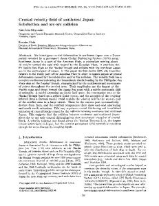
3. Three splines of t,hc type proposed in [5]. One apparent disadvantage to this approach is the difficulty in solving for the directions that provide continuity of curvature. Manning proposes an iterative approximation sclicmc that SCCIIIS to work well in practice, but he admits that thcrc is not always a unique solrtt,ion iuld Clicrc is 110 ~IliLrilIltCC thilt Chc itcrat,ion ;klWibyS convcrgcs to tllc dcsircti Sobtion. Cubic splints often have very low curvature at their endpoints when Ihcy have very sharp bends internally, and this can introduce cxtrancous solutions as shown in Figure 3. The three curves shown are all curvature continuous open curves that have given directions at x0 cand 22, but regardless of the initial conditions, Manning’s iteration always converges to one of the asymmetrical ones with sharp bends. If ~(1 is raised and 22 lowered until the angle x()zlz2 is about 122’, the ~asymnlctricnl solutions mcrgc with the symmetrical ones ;and the rate of convcrgcncc for Manning’s iteration approaches zero, While these kinds of problcnls do not seem to occur when the angles involved arc not 4

so large, much additional testing would be necessary in order to verify this. In section 3, we show how all such problems can be avoided by setting up a system of linear equations that are easy to solve Cand guarantee approximate continuity of curvature. We derive the specific equations appropriate for the fantily of curves discussed ir; Section 2, but similar equations could be derived for many different classes of curves. 2. The Magnitudes of the Velocity Vectors The subproblem to be solved in this section can be stated as follows: Given two points x; and zi+l, and two unit vectors wi and w;+l, find Can aesthetically pleasing parametric cubic z(t) so that z(0) = zi, z(1) = zi+l, z’(O) = cyw;, an’d z’(1) = pw;+l, w h e r e a! and ,B are positive real numbers and z’(t) is the componentwise derivative (z’(t), y’(t)) of 1 so wish to introduce two “tension” parameters T; and ?;+I such z(t) = (X(t),Y(Q). w e J that plcasing curves will be obtained when r; = ?fi+l = 1, and as the tensions approach 00, the curves will approach the line segment joining x; to zi+l. In order to guarantee that the results are independent of translation, rotation, and scaling, we shall begin by finding a function 2(t) such that 2(o) = (o,o),

i(l) = (l,O),

i’( o )

=

7;

$

I(&

4 )

l

(cos 8, sine),

a n d Z’(l) =

k

i

o

(e,4

)

+0~ 4

, ~ i n 4

)

(I)

where p and CT Care positive real functions to be determined later, 0 = arg w; -arg(zi+l -zi), and 4 = arg(z;+l -zi) -+arg w;+l. (Here arg(s, y) is the angle w such that (2, y) is a positive multiple of (cos w, sin w).) We then set

.(

4) = 2; +

Zl -20 Yo -Y1 Yl - Yo Xl--X0 >

a(t).

(21

It is not hard to set that the parametric cubic satisfying (1) has BCzicr control points (O,O), (p/3~;). (cos&sin0),-(1 - (a/3?;+1)cos4,(0/3;i;+l)sin4), and (l,O), so that E(t)

=

%(I

Ti

- t)2(C0d,sid) +

t2(1 - t)

(

3 - &, * + t3( 1,o). %+1 %+1 >

(3)

It only remains to choose positive functions p(0, 4) and a(O,4) so that ~(0, 4) = a(+, 0) = Pp, -4). In [5] M n, 0 < 0, and 0 # -4 SO as to avoid any possibility of generating a curve with a cusp in it. (This only effects the above functions when 4 >. 145”.) It is desirable to have a sitnplcr approximation that does not use transcendental functions other than sines ‘and cosines of 0 and 4. One such approximation is the following functions which were developed for the new METRFONT system [4]: 2+(3

1

p= i-t(i-c)cose+ccO~~' 2--a! O= l+(l-c)cos~+ccose~

where

a = u(sin 0 - 6 sin +)(sin 4 -- 6 sin U)(cosU - cos 4). The constants a, 6, and c were chosen to minimize an error function based on the value of (10) for 116 different (0, 4) pairs. This suggested a = 1.597, 6 = .0700, and c = .370, but since empirical evidcncc indicated that large values for ]p - CT] were causing problems, METAFONT uses the slightly pcrturbcd values a = a, 6 = -$, and c = (3 - &)/2. Figure 8 shows some of the curves gcncratcd by (9) and (10). They arc similar for moderate angles, but the simpler equations set /I too small and CY too large when, 4 = -90’. Equation (10) d oes not perform well in such extreme casts because it does not allow p - CT 9

8b. Curves from (10) with 0 = 45O.

8a. Curves from (9) with 0 = 45’.

to be large enough when 0 < 0/+ < 1 without making (T - p too large when -1 < e/4 < 0 or moving the cross-over point where p = CT too close to e/4 = 0. . 3. Mqck Curvature Constraints Here we need to.extend the notation of Section 2 SO that 0j = arg wj - arg(zi+r - zj) for 0 < j < 7Z, #j = arg(Zj - zj-1) - iL;Tg wj for 0 < j < n, and dj is the Euclidean length of the vector xj+r -zj for 0 2 j < n. If the problem is to find a closed curve with no directions given, it will be convenient to sometimes use alternative names z,+r, 8,, +n+r, T,, and ?n+r for xl, 80, +r,r(), and 71 respectively. We can then define $j’= arg(zj+l-zj)-~~g(zj-zj-~) for 1 < j 5 n’, where n’ = n for closed curve problems with no directions given and n' = n - 1 otherwise. Unless stated otherwise, all $j care at most 180” in absolute value. Where 20; has been given in advance, it simply determines 4; and 8;; other wi need to be determined by solving for & and 4i. Since the problem of finding direction angles can be broken into independent subproblems separatatcd by knots where directions are given, we can cassume that no directions other than 200 and w, are given. For closed curve . problems we can assume that no directions at all are given, otherwise the problem could be reduced to one or more open curve problems. The requirement that the curvature be continuous at some knot zi, 0 < i < n, is kl(~i-~,zi,wi-l,wi,~i-l)~i) z k()(zi,zi+l,wi,wi+l,ri,~i+l) where k. and ICI are functions that give the curvature at t = 0 and t = 1 in terms of the endpoints, terminal directions, ,and tension parameters for the family of curves being used. Because of the requirement for invariance under translation, rotation, and scaling, there , exists a function k such that I

-* ) = k(Oj,4j+l,Tj, Tj+l)/dj a n d kO(zj, zj+l,w j)wj+l, rj, rj+l kl (zj, zj+l, W*j 9Wj+l,rj, -* r34 1 ) z k(Sj.,.l) Oj, Tj+l; rj)/clje

(11)

Any particular family of curves determines a specific function k that satisfies (11). The corresponding lnock curv~ture function i consists of the linear terms in the Taylor series for k(O,q5, r , ?), expanded about (O,+) = (0,O). For the curves detcrmincd by (2) and (3) with p and CT determined by (9) or (lo),

and

j I

10

.

(12) where the angles are measured in radians. Since the tension parameters are always known in advance, they are treated like constants in this expansion. Continuity of mock curvature requires G-1)/4-l - i(t);, 4i+l, Ti, ?i+l)/d; = 0 i(4i’ k -1, C’

for 1 < i < n’.

(13)

Combining this with the first order continuity equations

ei + 4; =

-$i

for 1 5 i < n’

gives enough equations to determine all Bi and 4i for closed curve problems. For open curve problems when directions wo = xoq41,Qo’ %7-o)

The curl parameters give the ratio of the mock curvature at the endpoints to that at the adjacent knots. They should probably have default values of 1 so that the first and last spline segments will usually be good approximations to circular arcs as in Figure 9b. We now have a system of equations consisting of (In), (l/i>, and possibly (15~) and/or (156). If B. or 4n have been given in advance then they may bc regarded ras constants. The first step is to rewrite (15~) ,(156) as

;ud

so that 00 and 4n can be eliminated. Then (14) may be used to eliminate all 4i so that the remaining vsriablcs are Or, 02, . . . , O,,, and the remaining equations are those given by (13) with appropriate substitutions. This system has some important properties that may bc summarized cas follows.. 11

Theorem I. If n 2 2, if all tension parameters satisfy the bound ri, 7i 1 r,,in > $, and if any curl parameters satisfy ~0, xn 1 0, then cafter the aforementioned substitutions, a21 coefEcients in (13) are nonnegative, and for each i, the coefficient of ej 1 times the sum of all the other coefficients in that equation. is at Ieast 37,,,iIl -

0f el, ear . . . , enI

Proof. The bounds on the tension parameters guarantee that the coefficient of 8 in (12) will be negative, the coefficient of 4 will be positive, and the magnitude of the former will be at least 37en - 1 times the latter. When 1 < i < n’ in (13), the only relevant substitutions are 4j = -$j - 4j for 1~’ - iI 5 1, so the coefficients of 8;-1, Bi and 0i+r clearly have the required properties. For closed curve problems, the same holds for i = 1 and i = n’, otherwise additional substitutions eliminate 00 and 4n so that k(41,00, ?I, TO) depends only on 41 and &,_r,+,,r+r&) depends only on 8,-r. We need only show that both of these variables have non-positive coefhcients. This is clearly true for given directions, and it also holds for curl constraints since the coefficients in (16) are at most 370 - 1