Smooth Linear Approximation of Non-overlap Constraints Graeme Gange1 , Kim Marriott2 , and Peter J. Stuckey1,3 1
2
Department of Comp Sci and Soft Eng University of Melbourne, 3010, Australia
[email protected] Clayton School of IT Monash University, 3800, Australia
[email protected] 3 National ICT Australia, Victoria Laboratory
[email protected]
Abstract. Constraint-based placement tools and their use in diagramming tools has been investigated for decades. One of the most important and natural placement constraints in diagrams is that their graphic elements do not overlap. However, non-overlap of objects, especially nonconvex objects, is extremely difficult to solve, especially to solve sufficiently rapidly for direct manipulation. Here we present the first practical approach for solving non-overlap of possibly non-convex objects in conjunction with other placement constraints such as alignment and distribution. Our methods are based on approximating the non-overlap constraint by a smoothly changing linear approximation. We have found that this in combination with techniques for lazy addition of constraints, is rapid enough to support direct manipulation in reasonably sized diagrams.
1
Introduction
Diagram editors were one of the earliest applications areas for constraint-solving techniques in computing [22]. Constraint solving allows the editor to preserve design aesthetics, such as alignment and distribution, and structural constraints, such as non-overlap between objects, during manipulation of the graphic objects. The desire for real-time updating of the layout during user interaction means that fast incremental constraint solving techniques are required. This, and the difficult, non-linear, combinatorial nature of some geometric constraints, has motivated the development of many specialized constraint solving algorithms. Geometric constraint solving techniques have evolved considerably and modern diagram editors, such as MicrosSoft Visio and ConceptDraw, provide placement tools that impose persistent geometric constraints on the diagram elements, such as alignment and distribution. However, the kind of constraints provided is quite limited and, in particular, does not include automatic preservation of non-overlap between objects. This is, perhaps, unsurprising since solving nonoverlap constraints is NP-hard. Here we address the problem of how to solve nonoverlap constraints in conjunction with alignment and distribution constraints
Fig. 1. An example of non-overlap interacting with alignment. Each word is aligned horizontally, and no letter can overlap another. Starting from the left position direct manipulation of the letters updates the position of all objects in real time as letters are dragged around to reach the right position.
(a)
(b)
(c)
Fig. 2. Dynamic linear approximation of non-overlap between two boxes. Satisfaction of any of the constraints: left-of, above, below and right-of is sufficient to ensure nonoverlap. Initially (a) the left-of constraint is satisfied. As the left rectangle is moved (b), it passes through a state where both the left-of and above constraint are satisfied. When the left-of constraint stops the movement right, the approximation is updated to above and (c) motion can continue.
sufficiently quickly to support real-time updating of layout during user interaction. We have integrated our non-overlap constraints into the constraint based diagramming tool Dunnart. An example of using the tool is shown in Figure 1. The key to our approach is the use of dynamic linear approximation (DLA) [16, 12]. While many geometric constraints, such as alignment and distribution are linear, non-overlap is inherently non-linear. In DLA, non-linear constraints are approximated by linear constraints. In a specialization of this technique, smooth linear approximation (SLA), as the solution changes the linear approximation is smoothly modified. The approach is exemplified in Figure 2. Efficient incremental solving techniques for linear constraints [1] mean that this approach is potentially fast enough for interactive graphical applications. It is worth pointing out that SLA is not designed to find a new solution from scratch, rather it takes an existing solution and continuously updates this to find a new locally optimal solution. This is why the approach is tractable and also well suited to 2
interaction since, if the user does not like the local optimum the system has found, then they can use direct manipulation to escape the local optimum. Previous research has described a number of proof-of-concept toys that demonstrate the usefulness of SLA for non-overlap of two simple shapes, axis-aligned rectangles and circles. In this paper we extend this to provide the first systematic investigation of how to use SLA to handle non-overlap between arbitrary polygons of fixed sized and orientation. Handling convex polygons is a relatively straightforward extension from axis aligned rectangles. A single linear constraint between each pair of objects suffices to ensure non-overlap. Handling non-convex polygons is considerably more difficult and the main focus of this paper. The first approach (described in Section 5.1) is to decompose each non-convex polygon into a collection of convex polygons joined by equality constraints. Unfortunately, this leads to a large number of linear constraints between each pair of non-convex polygons since if these are decomposed into m and n convex polygons, respectively, then this gives rise to to mn constraints. In our second approach (described in Section 5.2), we invert the problem and, in essence, model non-overlap of polygons A and B by the constraint that A is contained in the region that is the complement of B. As we have described them, the above two methods are conservative in the sense that for each pair of objects there is always a linear constraint in the solver ensuring that the objects will not overlap. However, if the objects are not near each other this incurs the overhead of keeping an inactive inequality in the linear solver. We also investigate non-conservative, lazy, variants of the above two methods in which the linear constraints are added only if the objects are “sufficiently” close and removed once they are sufficiently far apart. These utilize fast collision-detection algorithms [14]4 and are described in Section 6. We provide a detailed empirical evaluation of these different approaches and their variants in Section 7. We find that SLA using the inverse approach with lazy addition of constraints is the fastest technique. Furthermore, it is very fast and fast enough to support immediate updating of object positions during direct manipulation for practically sized diagrams. We believe the algorithms described here provide the first viable approach to handling non-overlap of (possibly nonconvex) polygons in combination with other constraints in constraint-based diagramming tools.
2
Related Work
Starting with Sutherland [22], there has been considerable work on developing constraint solving algorithms for supporting direct manipulation in interactive graphical applications. These approaches fall into four main classes: propagation 4
It is perhaps worth emphasizing that collision-detection algorithms by themselves are not enough to solve our problem. We are not just interested in detecting overlap: rather, we must ensure that objects do not overlap while still satisfying other design and structural constraints and placing objects as close as possible to the user’s desired location.
3
based (e.g. [23]); linear arithmetic solver based (e.g. [3]); geometric solver-based (e.g. [13]); and general non-linear optimisation methods such as Newton-Raphson iteration (e.g. [17]). However, none of these techniques support non-overlap. Non-overlap constraints have been considered by Baraff [2] and Harada, Witkin, and Baraff [10], who use a specialised force based approach, modelling the non-overlap constraint between objects by a repulsion between them if they touch. However, they do not consider non-overlap constraints in conjunction with other linear constraints. Hosobe [11] describes a general purpose constraint solving architecture that handles non-overlap constraints and other non-linear constraints. The system uses variable elimination to handle linear equalities and a combination of non-linear optimisation and genetic algorithms to handle the other constraints. Our approach addresses the same issue but is technically quite different, and we believe much faster. The most closely related work are our earlier papers introducing DLA [16, 12]. The present paper extends these by providing a more detailed investigation of non-overlap and, in particular, of non-overlap of non-convex polygons. The algorithms given here to compute the linear approximation are all new.
3
Background: Smooth Linear Approximation
In constraint-based editors the author can place geometric constraints on the objects in the diagram. During subsequent editing these geometric constraints will be maintained until the user explicitly removes them. Standard geometric constraints are: • horizontal and vertical alignment • horizontal and vertical distribution • horizontal and vertical ordering that keeps objects a minimum distance apart horizontally or vertically while preserving their relative ordering • an “anchor” tool that allows the user to fix the current position of a selected object or set of objects. Each of the above geometric relationships can be modelled as a linear constraint over variables representing the position of the objects in the diagram. For this reason, a standard approach in constraint-based graphics editors is to use a constraint solver that can support arbitrary linear constraints. Direct manipulation is handled as follows. Assume that the variables y1 , ..., ym correspond to objects which are the subject of the direct manipulation and that the variables x1 , ..., xn correspond to the remaining objects, and let C be the set of linear constraints representing geometry constraints. During directly manipulation the system successively solves a sequence of linear optimization problems of the form: Pm Pn Minimize ws i=1 |xi − ci | + we i=j |yj − dj | subject to C where ci is the current value of xi and dj is the desired value of yj . The weighting constants ws and we specify how important it is to move the yj ’s to their desired 4
position as opposed to leaving the xi ’s at their current position. Typically we is much greater than ws . The effect of the optimization is to move the objects being directly manipulated to their desired value, i.e. where the user wishes to place them, and leave the other objects where they are unless they are connected by constraints to the objects being moved. This optimization problem is repeatedly resolved during direct manipulation for different values of the di ’s. Fast incremental algorithms have been developed to do this so that the object positions can be updated in real-time [1]. However, not all geometric constraints are linear. Dynamic linear approximation (DLA) [16, 12] is a recent technique for handling non-linear constraints that builds upon the aforementioned efficient linear constraint solving algorithms. In DLA, non-linear constraints are approximated by linear constraints. Consider a complex constraint C. A linear approximation of a complex constraint is a (possibly infinite) disjunctive set of linear configurations {F0 , F1 , . . . } where each configuration Fi is a conjunction of linear constraints. For example for the non-overlap constraint of the two boxes in Figure 2 there are four configurations left-of, above, below and right-of each consisting of a single linear constraint. We require that the linear approximation is safe in the sense that each linear configuration implies the complex constraint and complete in the sense that each solution of C is a solution of one of the linear configurations. For the purposes of this paper we will consider the complex constraint C to be a disjunctive set of its linear configurations. In a specialization of this technique, smooth linear approximation (SLA), as the solution changes the linear approximation is smoothly modified. SLA works by moving from one configuration for a constraint to another, requiring that both configurations are satisfied at the point of change. This smoothness criteria reduces the difficulty of the problem substantially since we need to consider only configurations that are satisfied with the present state of the diagram. It also fits well with continuous updating of the diagram during direct manipulation. The initial approach to smooth linear approxiation [16] involved keeping all disjunctive configurations in the underlying linear solver, and relying on the solver to switch between disjunctions. This has a number of problems: the number of configurations must be finite, and there is significant overhead in keeping all configurations in the solver. This was improved in [12] by storing only the current configuration in the solver and dynamically generating and checking satisfiability of other configurations when required. The basic generic algorithm for solving a set of smooth linear approximations is given in Figure 3. kim[Should this solve after each configuration change?] Given a set of complex constraints C and their current configurations F as well as an objective function o to be mininimized, the algorithm uses a linear constraint solver to find an minimal solution θ with the current configuration. It then searches for alternative configurations that are satisfied currently, but if replaced would allow the objective function to decrease further. The algorithm 5
sla(C, F, o) Let C = {C0 , C1 , ..., Cn } be the set of complex constraints. Let F = {F0 , F1 , ..., Fn } be the current set of configurations. repeat V θ := minimize o subject to n j=1 Fj finished := true for i ∈ 1..n V Fi0 = update(θ, Ci , Fi , n j=1,j6=i Fj , o) if Fi 6= Fi0 then Fi := Fi0 finished := false until finished update(θ, C, F, F, o) if ∃F 0 ∈ C where F 0 6= F and θ satisfies F 0 and F 0 will improve the solution return F 0 else return F
Fig. 3. General algorithm for solving sets of smooth linear approximations.
repeatedly replaces configurations until no further improvement is possible. The algorithm is generic in: – The choice and technique for generating the linear configurations for the complex constraint. – How to determine if an alternative linear configuration might improve the solution. In the next two sections we describe various choices for these operations for modelling non-overlap of two polygons.
4
Non-overlap of convex polygons
Smooth Linear Approximation (SLA) is well suited to modelling non-overlap of convex polygons. The basis for our approach is the Minkowski difference, denoted by P ⊕ − Q, of the two polygons P and Q we wish to ensure do not overlap. Given some fixed point pQ in Q and pP in P the Minkowski difference is the polygon M s.t. the point pQ − pP (henceforth referred to as the query point) is inside M iff P and Q intersect. For convex polygons, it is possible to “walk” one polygon around the boundary of the second; the vertices of the Minkowski difference consist of the offsets of the second polygon at the extreme points of the walk. It follows that the Minkowski difference of two convex polygons is also convex. An example of the Minkowski difference of two convex polygons is given in Figure 4 while an example of a non-convex Minkowski sum is shown in Figure 5. 6
11111111111 00000000000 00000000000 11111111111 00000000000 11111111111 00000000000 11111111111 00000000000 11111111111 00000000000 11111111111 00000000000 11111111111 00000000000 11111111111 00000000000 11111111111 00000000000 11111111111 00000000000 11111111111 00000000000 11111111111 00000000000 11111111111 00000000000 11111111111 00000000000 11111111111 00000000000 11111111111 00000000000 11111111111 00000000000 11111111111 00000000000 11111111111 00000000000 11111111111
Fig. 4. A unit square S and unit diamond D and their Minkowski difference S ⊕ −D. The local origin points for each shape are shown as circles.
There has been considerable research into efficient computation of the Minkowski difference of two polygons.5 Optimal O(n + m) algorithms for computing the Minkowski difference of two convex polygons with n and m vertices have been known for some time [8, 18]. Until recently calculation of the non-convex Minkowski difference decomposed the polygons into convex components, constructed the convex Minkowski difference of each pair, and took the union of the resulting differences. Recently direct algorithms have appeared based on convolutions of a pair of polygons [19, 6]. We make use of the implementations in the CGAL (www.cgal.org) computational geometry library. We can model non-overlap of convex polygons P and Q by the constraint that the query point is not inside their Minkowski difference, M . As the Minkoskwi difference of two convex polygons is a convex polygon, it is straightforward to model non-containment in M : it is a disjunction of single linear constraints, one for each side of M , specifying that the query point lies on the outside of that edge. Consider the unit square S and unit diamond D shown in the left of Figure 4. Their Minkowski difference is shown in the right of Figure 4. The linear approximation of the non-overlap constraint between S and D is the disjunctive configuration: {y ≤ 0, x+y ≤ 0, x ≤ 0.5, y −x ≥ 2, y ≥ 2, x+y ≥ 3, x ≤ 1.5, y −x ≤ −1} which represent the 8 sides of the Minkowski difference shown at the right of the figure, from the bottom in clockwise order, where (x, y) = (xD , yD ) − (xS , yS ) represents the relative position of the diamond to the square. The approximation is conservative and accurate. It is also relatively simple and efficient to update the approximation as the shapes are moved. Note that the Minkowski difference only needs to be computed once. However before getting into details of how to update the approximation, we need to introduce Lagrange 5
More precisely, research has focussed on the computation of their Minkowski sum since the Minkowski difference of A and B is simply the Minkowski sum of A and a reflection of B.
7
multipliers. These are a fundamental notion in constrained optimization, but describing their properties is beyond the scope of this paper; the interested reader is referred to [7]. Here, it suffices to understand that the value of the Lagrange Pn multiplier λc for a linear inequality c ≡ i=1 ai xi ≤ b provides a measure of how “binding” a constraint is; it gives the rate of increase of the objective function as a function of the rate of increase of b. That is, it gives the cost that imposing the constraint will have on the objective function, or conversely, how much the objective can be increased if the constraint is relaxed.6 Thus, intuitively, a constraint with a small Lagrange multiplier is preferable to one with a large Lagrange multiplier since it has less effect on the objective. In particular, removing a constraint with a Lagrange multiplier of 0 will not allow the objective to be improved and so the Lagrange multiplier is defined to Pn be 0 for an inequality that is not active, i.e. if i=1 ai xi < b. Simplex-based linear constraint solvers, as a byproduct of optimization, compute the Lagrange multiplier of all constraints in the solver. Updating of the linear approximation to non-overlap with a convex polygon works as follows. Assume that the current linear approximation is the linear constraint c corresponding to boundary edge e and that the current solution is θ. If λc = 0 we need do nothing since changing the constraint could not improve the solution. Otherwise assume that λc > 0. We consider the two edges e1 and e2 adjacent to e and their corresponding constraints c1 and c2 . If θ does not satisfy c1 and does not satisfy c2 , then we do not change the choice of linear approximation since it cannot be done smoothly. Otherwise, it will satisfy at most one of the two, say c1 . We must now determine if it will improve the solution if we swap c for c1 . We do this by tentatively adding c1 to the solver and computing its Lagrange multiplier λc1 . (Note that this is very efficient since the current solution will still be the optimum.) If λc1 < λc then we are better off swapping to use c1 . This is done by removing c from the solver, leaving c1 in the solver. Otherwise, we are better off staying with the current approximation, so we remove c1 from the solver.
5
Non-Convex Polygons
We now give two extensions of our technique for handling non-overlap of convex polygons to the case when one or both of the polygons are non-convex. We do not allow holes in the polygons. kim[But could] 5.1
Decomposition into convex polygons
Probably the most obvious approach is to simply decompose the non-convex polygons into a union of convex polygons which are constrained to be joined together (either using equality constraints, or simply using the same variables 6
It follows that at an optimal solution the Lagrange multiplier λc for an inequality cannot be negative.
8
111111 000000 000000 111111 000000 111111 000000 111111 000000 111111 000000 111111 000000 111111 Fig. 5. The Minkowski difference of a non-convex and a convex polygon. From left, A, B, extreme positions of A and B, A ⊕ −B.
to denote their position), and add a non-overlap constraint for each pair of polygons. This decomposition based method is relatively simple to implement since there are a number of well explored methods for convex partitioning of polygons, including Greene’s [9] dynamic programming method for optimal partitioning. However, it has a potentially serious drawback: in the worst case, even the optimal decomposition of a non-convex polygon will have a number of convex components that is O(n) where n the number of vertices in the polygon. This means that in the worst case the non-overlap constraint for each pair of nonconvex polygons with O(n) vertices will lead to O(n2 ) non-overlap constraints between the convex polygons. 5.2
Inverse Approach
However, in reality most of these Ω(n2 ) constraints are redundant and unnecessary. An alternative approach is to use our earlier observation that we can model non-overlap of convex polygons P and Q by the constraint that the query point is not inside their Minkowski difference, M . This remains true for non-convex polygons, although the Minkowski difference may now be non-convex. An example Minkowski difference for a non-convex polygon is shown in Figure 5. In our second approach we pre-compute the Minkowski difference M of the two, possibly non-convex, polygons P and Q and then decompose the space not occupied by the Minkowski polygon into a union of convex regions, R1 , .., Rm . We have that the query point is not inside M iff it is inside one of these convex regions. Thus, we can model non-overlap by a disjunction of linear constraints, with one for each region Ri , specifying that the query point lies inside the region. We call this the inverse approach. Since the original polygons are not allowed to contain holes, their Minkowski difference will be also be a simple polygon without holes. kim[Rubbish!] This can be described by the polygon’s convex hull and a series of non-convex pockets where the boundary of the polygon deviates from the convex hull. The key to the 9
Fig. 6. A non-convex polygon, together with convex hull, decomposed pockets and adjacency graphs. From a given region, the next configuration must be one of those adjacent to the current region.
inverse approach is that whenever the query point is not overlapping with the polygon, it must be either outside the convex hull of the polygon (as in the convex case), or inside one of the pockets. If each pocket is then partitioned into convex regions, it is possible to approximate the non-overlap of two polygons with either a single linear constraint (for the convex hull) or a convex containment (for a pocket region). An example is shown in Figure 6 As the desired goal is to reduce the number of constraints in the linear constraint solver, it seems reasonable to partition the pockets into triangular regions, resulting in at most 3 constraints per pair of polygons. The use of a triangulation has the added benefit of defining an adjacency graph which allows selection of adjacent regions in O(1) time (Figure 6). There are a number of algorithms for partitioning simple polygons into triangles [21, 4], of varying complexity; the present implementation uses a simple approach described by O’Rourke [18]. One of the advantages of the inverse approach is that, in most cases, particularly when the pairs of polygons are distant, the two polygons are treated as convex. It is only when the polygons are touching, and the query point lies upon the opening to a pocket that anything more complex occurs. Updating of the approximation extends that given earlier for convex polygons. The new case is that the current linear approximation is one of the triangular regions, R, in the pocket. In this case it has three constraints c1 , c2 , c3 corresponding to each boundary edge. We have pre-computed the subset of those constraints that correspond to boundary constraints that are permeable in the sense that the boundary is shared with the convex hull or another triangular region. We compare the Lagrange multipliers of these constraints and determine which constraint has the largest Lagrange multiplier, say c. If λc = 0 we need do nothing since changing the region cannot improve the solution. Otherwise the current solution is on the boundary corresponding to c and so we move to the adjacent region sharing the same boundary.
6
Lazy Addition of Constraints
The preceding methods are all conservative in the sense that for each pair of objects there is always a linear constraint in the solver ensuring that the objects will not overlap. However, if the objects are not near each other this incurs the 10
overhead of keeping an inactive inequality in the linear solver. A potentially more efficient approach is to lazily add the linear constraints only if the objects are “sufficiently” close and remove them once they are sufficiently far apart. We have investigated two variants of this idea which differ in the meaning of sufficiently close. The first method measures closeness by using the bounding boxes of the polygons. If these overlap, a linear approximation for the complex constraint is added and once they stop overlapping it is removed. We also investigated a more precise form of closeness, based on the intersection of the actual polygons, rather than the bounding box. However, we found the overhead involved in detecting intersection and the instability introduced by repeatedly adding and removing the non-overlap constraint made this approach infeasible. Thus we focus on the first variant. Implementation relies on an efficient method for determining if the bounding boxes of the polygons overlap. Determining if n 2-D bodies overlap is a well studied problem and numerous algorithms and data structures devised including Quad/Oct-trees [20], and dynamic versions of structures such as range, segment and interval-trees [5]. Unfortunately many of these methods handle nonrectangular shapes poorly, or are very difficult to implement. The method we have chosen to use is an adaptation of that presented in [14]. The algorithm is based, as with most efficient rectangle-intersection solutions, on the observation that two rectangles in some number of dimensions will intersect if and only if the span of the rectangles intersect in every dimension. Thus, maintaining a set of interacting rectangles is equivalent to maintaining (in two dimensions) two sets of intersecting intervals. The algorithm acts by first building a sorted list of rectangle endpoints, and marking corresponding pairs to denote whether or not they are intersecting in either dimension. While this step takes, in the worst case O(n2 ) time for n rectangles, it is in general significantly faster. As shapes are moved, the list must be maintained in sorted order, and interacting pairs updated. This is done by using insertion sort at each time-step, which will sort an almost sorted list in O(n) time. Note that it is undesirable to remove the linear constraint enforcing nonoverlap between two polygons as soon as the solver moves them apart and their bounding boxes no longer intersect; instead, such pairs of polygons are added to a removal buffer, and then removed only if their bounding boxes are still not intersecting after the solver has reached a stable solution. A change in intersection is registered only when a left and right endpoint of different bounding boxes swap positions. If a left endpoint is shifted to the left of a right endpoint, an intersection is added if and only if the boxes are already intersecting in all other dimensions. If a left endpoint is shifted to the right of a right endpoint, the pair cannot intersect, so the pair is added to the removel buffer (if currently intersecting). (See Figure 7) Unfortunately, we have found that this simple approach to lazy (or late) addition of constraints has the significant drawback of violating the conservativeness of the approximation and somewhat undermines the smoothness of the approxi11
b1
b2
e1
e2 b3
b4
e3
e4
b1
e1 b2
b3
e2
b4
e3
e4
Fig. 7. The sorted list of endpoints is kept to facilitate detection of changes in intersection. As the second box moves right, b2 moves to the right of e1 , which means that boxes 1 and 2 can no longer intersect. Conversely, endpoint e2 moves to the right of b3 , which means that boxes 2 and 3 may now intersect.
mation since objects can momentarily overlap during direct manipulation. This can cause problems when the objects are being moved rapidly; that is, the distance moved between solves is large compared to the size of the objects. This is not very noticeable with the inverse approach but is quite noticeable with the decomposition method, as the convex components (and hence bounding boxes) are often rather small; if two shapes are moved sufficiently far between solves, the local selection of configurations may be unsatisfiable. One possible solution would be to approximate the shapes by a larger rectangle with some “padding” around each of the objects. Another possible approach is to use rollback to recover from overlapping objects. When overlap is detected using collision detection, we roll back to the previous desired values (which did not lead to overlap), add the non-overlap constraint and re-solve and, finally, solve for the current desired value. This should maintain most of the speed benefits of the current lazy addition approaches, while maintaining conservativeness of approximation; and using a separate layer for the late addition avoids adding additional complexity to the linear constraint solver.
7
Evaluation
The algorithms were implemented using the Cassowary linear inequality solver, included with the QOCA constraint solving toolkit [15]. Non-convex Minkowski difference calculation was implemented using the Minkowski sum 2 CGAL package produced by Wein [24]. We implemented both the decomposition and inverse approach for handling non-overlap of non-convex polygons. The decomposition was handled using Greene’s dynamic programming algorithm [9]. For each version, both the conservative and lazy versions were implemented for comparison, and (of course) executed with exactly the same input sequence of interaction. Two experiments were conducted. Both involved direct manipulation of diagrams containing a large number of non-convex polygons some of which were linked by alignment constraints. We focussed on non-convex polygons because all of our algorithms will be faster with convex polygons than non-convex. The 12
(a)
( b)
Fig. 8. Diagrams for testing. (a) Non-overlap of polygons representing text. The actual diagram is constructed of either 2 or 3 repetitions of this phrase. (b) The top row of shapes is constrained to align, and pushed down until each successive row of shapes is in contact.
experimental comparison of the approaches were run on an Intel Core2 Duo E6700 with 2GB RAM. The first experiment measured the time taken to solve the constraint system for a particular set of desired values during direct manipulation of the diagram containing non-convex polygons representing letters, shown in Figure 8(a). Individual letters were selected and moved into the center of the diagram in turn. The results are given in Table 1(a). Note that the conservative decomposition method was unusable on the full diagram with 3 copies of the text, this is indicated with “–” in the table entry. On a smaller version of the diagram with 2 copies of the text it took on average 107 milliseconds. In order to further explore scalability, a diagram of tightly fitting U-shapes, Figure 8(b), of a varying number of rows was constructed, and the top row pushed through the lower layers. Results are given in Figure 1(b).
Direct Inverse Rows Cons Lazy Cons Lazy 5 16.99 1.86 2.79 0.87 Ave Time 6 34.95 2.21 2.93 1.23 Max Time 7 23.12 4.13 4.99 1.49 Ave Cycle 8 34.35 4.05 7.01 2.02 Max Cycle 9 49.02 7.40 10.99 2.51 10 61.90 7.68 12.07 5.39 (a) Text diagram (b) U-shaped polygons Table 1. Experimental results. For the text diagram, we show the average and maximum time to reach a stable solution, and the average and maximum number of solving cycles to stabilize. For the U-shaped polygon test we show average time to reach a stable solution as the number of rows increases. All times are in milliseconds. Direct Cons Lazy – 15.49 – 26.03 – 2.58 – 18
Inverse Cons Lazy 4.77 3.15 31.54 11.26 1.89 2.55 16 10
The results clearly demonstrate that the inverse approach is significantly faster than the decomposition approach. They also show that for both approaches the lazy versions are significantly faster than the conservative versions. Interest13
ingly, the conservative version of the inverse approach appears to outperform even the lazy version of the decomposition approach in cases where the convex hulls do not penetrate (such as the text example). Most importantly the results also demonstrate that the inverse approach (with or without laziness) can solve non-overlap constraints sufficiently rapidly to facilitate immediate update of polygon positions during direct manipulation of realistically sized diagrams.
8
Conclusions
We have explored the use of smooth linear approximation (SLA) to handle solving of non-overlap constraints between polygons. We presented two possible approaches for handling non-overlap of non-convex polygons and have shown that the inverse method (which models non-overlap of polygons A and B by the constraint that A is contained in the region that is the complement of B) is significantly faster than decomposing each non-convex polygons into a collection of adjoining convex polygons. We have also shown that the inverse method can be sped up by combining it with traditional collision-detection techniques in order to lazily add the nonoverlap constraint only when the bounding boxes of the polygons overlap. This is capable of solving non-overlap of large numbers of complex, non-convex polygons rapidly enough to allow direct manipulation, even when combined with other types of linear constraints, such as alignment constraints. Acknowledgements We thank Michael Wybrow for his help in integrating the non-overlap constraint solving code into the Dunnart diagramming tool and Peter Moulder and Nathan Hurst for insightful comments and criticisms.
References 1. Greg J. Badros, Alan Borning, and Peter J. Stuckey. The Cassowary linear arithmetic constraint solving algorithm. ACM Trans. Comput.-Hum. Interact., 8(4):267–306, 2001. 2. D. Baraff. Fast contact force computation for nonpenetrating rigid bodies. Proceedings of the 21st Annual Conference on Computer Graphics and Interactive Techniques, pages 23–34, 1994. 3. A. Borning, K. Marriott, P. Stuckey, and Y. Xiao. Solving linear arithmetic constraints for user interface applications. In Proceedings of the 10th annual ACM symposium on User Interface Software and Technology, pages 87–96. ACM Press New York, NY, USA, 1997. 4. B. Chazelle. Triangulating a simple polygon in linear time. Discrete and Computational Geometry, 6(1):485–524, 1991. 5. Yi-Jen Chiang and Roberto Tamassia. Dynamic algorithms in computational geometry. Proceedings of the IEEE, 80(9):1412–1434, 1992.
14
6. Eyal Flato. Robust and efficient construction of planar Minkowski sums. Master’s thesis, School of Computer Science, Tel-Aviv University, 2000. 7. R. Fletcher. Practical methods of optimization. Wiley-Interscience New York, NY, USA, 1987. 8. Pijush K. Ghosh. A solution of polygon containment, spatial planning, and other related problems using minkowski operations. Comput. Vision Graph. Image Process., 49(1):1–35, 1990. 9. D.H. Greene. The decomposition of polygons into convex parts. Computational Geometry, pages 235–259, 1983. 10. M. Harada, A. Witkin, and D. Baraff. Interactive physically-based manipulation of discrete/continuous models. Proceedings of the 22nd Annual Conference on Computer Graphics and Interactive Techniques, pages 199–208, 1995. 11. H. Hosobe. A modular geometric constraint solver for user interface applications. Proceedings of the 14th annual ACM symposium on User Interface Software and Technology, pages 91–100, 2001. 12. N. Hurst, K. Marriott, and P. Moulder. Dynamic approximation of complex graphical constraints by linear constraints. In Proceedings of the 15th annual ACM symposium on User Interface Software and Technology, pages 27–30, 2002. 13. G.A. Kramer. A geometric constraint engine. Artificial Intelligence, 58(1-3):327– 360, 1992. 14. M. Lin, D. Manocha, and J. Cohen. Collision detection: Algorithms and applications, 1996. 15. Kim Marriott, Sitt Chen Chok, and Alan Finlay. A tableau based constraint solving toolkit for interactive graphical applications. In Proceedings of the 4th International Conference on Principles and Practice of Constraint Programming, pages 340–354, London, UK, 1998. Springer-Verlag. 16. Kim Marriott, Peter Moulder, Peter J. Stuckey, and Alan Borning. Solving disjunctive constraints for interactive graphical applications. In Proceedings of the 7th International Conference on Principles and Practice of Constraint Programming, pages 361–376, London, UK, 2001. Springer-Verlag. 17. Greg Nelson. Juno, a constraint-based graphics system. In Proceedings of the 12th annual conference on Computer Graphics and Interactive Techniques, pages 235–243, New York, NY, USA, 1985. ACM Press. 18. Joseph O’Rourke. Computational Geometry in C. 2nd edition, 1998. 19. GD Ramkumar. An algorithm to compute the Minkowski sum outer-face of two simple polygons. Proceedings of the Twelfth Annual Symposium on Computational geometry, pages 234–241, 1996. 20. Hanan Samet. The Design and Analysis of Spatial Data Structures. 1990. 21. R. Seidel. A simple and fast incremental randomized algorithm for computing trapezoidal decompositions and for triangulating polygons. Comput. Geom. Theory Appl, 1(1):51–64, 1991. 22. Ivan E. Sutherland. Sketch pad a man-machine graphical communication system. In DAC ’64: Proceedings of the SHARE design automation workshop, pages 6.329– 6.346, New York, NY, USA, 1964. ACM Press. 23. B. Vander Zanden. An incremental algorithm for satisfying hierarchies of multiway dataflow constraints. ACM Transactions on Programming Languages and Systems (TOPLAS), 18(1):30–72, 1996. 24. Ron Wein. Exact and efficient construction of planar Minkowski sums using the convolution method. In Proceedings of the 14th Annual European Symposium on Algorithms, pages 829–840, September 2006.
15