knowledge in the statistical analysis of gene expression data. Advantages of .... regulated. However, the direction of regulation may be extracted as the sign of.
Statistical Applications in Genetics and Molecular Biology Volume 10, Issue 1
2011
Article 37
Smoothing Gene Expression Data with Network Information Improves Consistency of Regulated Genes Guro Dørum, Norwegian University of Life Sciences Lars Snipen, Norwegian University of Life Sciences Margrete Solheim, Norwegian University of Life Sciences Solve Saebo, Norwegian University of Life Sciences
Recommended Citation: Dørum, Guro; Snipen, Lars; Solheim, Margrete; and Saebo, Solve (2011) "Smoothing Gene Expression Data with Network Information Improves Consistency of Regulated Genes," Statistical Applications in Genetics and Molecular Biology: Vol. 10: Iss. 1, Article 37. DOI: 10.2202/1544-6115.1618
Brought to you by | Universitet for Miljoe & Biovitenskap Authenticated | 128.39.175.62 Download Date | 12/3/12 1:29 PM
Smoothing Gene Expression Data with Network Information Improves Consistency of Regulated Genes Guro Dørum, Lars Snipen, Margrete Solheim, and Solve Saebo
Abstract Gene set analysis methods have become a widely used tool for including prior biological knowledge in the statistical analysis of gene expression data. Advantages of these methods include increased sensitivity, easier interpretation and more conformity in the results. However, gene set methods do not employ all the available information about gene relations. Genes are arranged in complex networks where the network distances contain detailed information about inter-gene dependencies. We propose a method that uses gene networks to smooth gene expression data with the aim of reducing the number of false positives and identify important subnetworks. Gene dependencies are extracted from the network topology and are used to smooth genewise test statistics. To find the optimal degree of smoothing, we propose using a criterion that considers the correlation between the network and the data. The network smoothing is shown to improve the ability to identify important genes in simulated data. Applied to a real data set, the smoothing accentuates parts of the network with a high density of differentially expressed genes. KEYWORDS: differentially expressed genes, gene network, gene set analysis, microarray data analysis, enrichment analysis Author Notes: We would like to thank two anonymous referees for their help in improving this manuscript.
Brought to you by | Universitet for Miljoe & Biovitenskap Authenticated | 128.39.175.62 Download Date | 12/3/12 1:29 PM
Dørum et al.: Smoothing Gene Expression Data with Network Information
1 Introduction Gene Set Enrichment Analysis (Subramanian et al., 2005) and similar methods have in recent years become a popular way of evaluating gene expression data in light of background knowledge of gene sets. The fundamental idea is that sets of genes with some logical connection should show similarities with regard to expression level, and that differential expression should be evaluated at the gene set level instead of at the individual gene level. The benefit of this strategy may be a reduction in the number of false positives, since small, but consistent changes in expressions at the gene set level may be more reliable than large expression changes for individual genes. The sets of genes may be defined in different ways, but is of course motivated by the assumption of correlated expressions between the members of the set. Examples include metabolic pathways, functional categories and gene ontology levels. Various versions of gene set analysis methods have been proposed by Kim and Volsky (2005), Jiang and Gentleman (2007) and Efron and Tibshirani (2007). See Huang et al. (2009) for a recent review. It is however known that genes are arranged in complex networks, and gene set methods do not take full advantage of the information contained in these networks. Gene set methods require that the genes are divided into groups, while genes may take part in several reactions and do not necessarily fall into just one group. There may therefore be considerable overlap between groups. By shifting the focus from gene sets to gene networks, we can avoid the division into groups and at the same time make full use of the information about gene dependencies contained in the network distances. The fundamental idea is similar to the idea behind gene set methods, that there is a connection between network distance and gene expression similarity. A growing number of papers are describing methods that make use of detailed network information for the analysis of expression data. Vert and Kanehisa (2003) presented a method for correlating gene networks and gene expression data. ¨ Rahnenfuhrer et al. (2004) used distance between pairs of genes to improve statistical scores for finding active pathways. Hanisch et al. (2002) used information about gene networks to improve clustering of gene expression data. In regression modelling network information has also been used to smooth the estimated regression coefficients. Both Li and Li (2008) and Pan et al. (2010) used the network information as a penalization constraint in the parameter estimation, whereas Sæbø et al. (2008) used the network information to adjust the rotations in the Partial Least Squares regression model in their L-PLS. Shojaie and Michailidis (2009) incorporated network information in a latent variable model and used a mixed linear model framework to test the significance of subnetworks, with a generalisation (Shojaie and Michailidis, 2010) of the method to handle more complex experimental de1
Brought to you by | Universitet for Miljoe & Biovitenskap Authenticated | 128.39.175.62 Download Date | 12/3/12 1:29 PM
Statistical Applications in Genetics and Molecular Biology, Vol. 10 [2011], Iss. 1, Art. 37
signs and test several contrasts simultaneously. Rapaport et al. (2007) used network information to extract the relevant signals in the gene expression data by removing the high-frequency components, and adapted this to classification. Our approach is similar to the one in Rapaport et al. in that we aim at smoothing away the part of the gene expression data that represents noise. The goal is to eliminate false positives and accentuate important subnetworks with a high density of differentially expressed genes. The method is demonstrated on data simulated from one fictional and three real networks, and on a data set from a real experiment on Enterococcus faecalis.
2 Method In this section we describe the method of network smoothing. The procedure requires that some type of network information is available for the genes in the expression data. A matrix of distances between genes is extracted from the graph topology. We assume that network distances correspond to similarity between the genes’ expression patterns, and refer to this matrix as a similarity matrix. The similarity matrix is then used for smoothing of the gene expression data.
2.1
Similarity matrix
A predefined gene network, containing g genes, can be represented as a simple graph G, with genes as nodes and edges between genes representing some biological relationship. A simple graph is undirected, contains no loops and has at maximum one edge between each pair of nodes. Let i and j represent two nodes in G, and let i ∼ j indicate that the two nodes are adjacent (directly connected). The g × g adjacency matrix A describes the nodes’ neighbourhoods, and the entries ai j are { 1 if i ∼ j ai j = (1) 0 else for i, j = 1, 2, ..., g. The g × g degree matrix D is a diagonal matrix with the degree, i.e. the number of edges to a node, on the diagonal. Let δi be the degree of node i. The entries in D are { δi if i = j di j = (2) 0 else
DOI: 10.2202/1544-6115.1618
Brought to you by | Universitet for Miljoe & Biovitenskap Authenticated | 128.39.175.62 Download Date | 12/3/12 1:29 PM
2
Dørum et al.: Smoothing Gene Expression Data with Network Information
The g × g Laplacian matrix (Chung, 1997) is defined as L = D − A, where the entries are −1 if i ∼ j di j if i = j li j = (3) 0 else There are numerous ways of translating the network topology of G into similarity between genes. Here, we will focus on the diffusion kernel (Chung, 1997, Kondor and Lafferty, 2002) as a similarity measure. The concept of diffusion is closely related to random walks and can be imagined as information, just like a fluid, travelling through the network. The diffusion kernel, or diffusion matrix Sβ as we will refer to it here, is defined by the matrix exponential of L: −β L
Sβ = e
g
=
∑ vie−β λi vTi
(4)
i=1
where vi and λi are the i’th eigenvector and eigenvalue of L, respectively. Sβ depends on a parameter β , where β > 0, that controls the speed of diffusion through the graph. The diffusion is faster for larger values of β , corresponding to shorter distances between nodes. The diffusion matrix contains numbers between 0 and 1, and all rows and columns sum to 1. Figure 1 shows a fictional network and Figure 2 shows its diffusion matrix Sβ when the diffusion parameter β is set to 0.1 and 0.7, respectively. In the diffusion matrix black indicates values close to 0 and corresponds to long distances between nodes, and white indicates values close to 1 and corresponds to short distances. With β = 0.1 there are large distances also between the closely connected nodes, indicated by close to white diagonal elements and black off-diagonal elements. When β is increased to 0.7, the shorter distances between nodes is particularly apparent for the tightly connected nodes 1 to 6, indicated by the lighter area around these nodes. Node 17 is directly connected to only one node, and the colour of the diagonal element has not changed much from β = 0.1 to β = 0.7. The information has only one way of travelling to and from node 17, so it will remain mostly unaffected by an increase in the diffusion. Increasing β too much will eventually result in all connected genes getting an identical diffusion value. Since the purpose in this paper is to use the diffusion matrix for smoothing, we have chosen an upper limit on β by requiring that the diagonal should always contain the largest number in each row. This is equivalent to requiring that a node should always put most weight on itself. We refer to the upper limit as βmax . In section 2.3 we propose a measure for finding the optimal value of β between 0 and βmax .
3
Brought to you by | Universitet for Miljoe & Biovitenskap Authenticated | 128.39.175.62 Download Date | 12/3/12 1:29 PM
Statistical Applications in Genetics and Molecular Biology, Vol. 10 [2011], Iss. 1, Art. 37
9 8 10 7
11
3
5
27
12 26
6 4
1 2
25
13
24 14 23 18 15 19
16 17
20
Figure 1: Fictional network. 22
1
2
3
4
5
6
7
8
9
10 11 12 13 14 15 16 17
1
1
1
2
2
3
3
4
4
5
5
6
6
7
7
8
8
9
9
10
10
11
11
12
12
13
13
14
14
15
15
16
16
17
17
(a) β = 0.1
2
3
4
5
6
21
7
8
9
10 11 12 13 14 15 16 17
(b) β = 0.7
Figure 2: Graphical representation of the diffusion matrix for the fictional network. Black indicates large distances and white indicates small distances.
DOI: 10.2202/1544-6115.1618
Brought to you by | Universitet for Miljoe & Biovitenskap Authenticated | 128.39.175.62 Download Date | 12/3/12 1:29 PM
4
Dørum et al.: Smoothing Gene Expression Data with Network Information
2.2
Smoothing expression data
Let X denote an n × g matrix of gene expression levels measured for g genes on n samples. A test statistic, e.g. a t-statistic for testing differential expression between two conditions, correlation between the gene and a phenotype vector or a signal-tonoise ratio, is calculated for each gene. Let t denote the g×1 vector of test statistics. The absolute values of the test statistics are multiplied with the diffusion matrix Sβ to obtain a vector of smoothed test statistics tβ : tβ = Sβ |t|
(5)
The diffusion matrix acts like a weighting matrix since each row sums to 1. The smoothing will give closely connected genes a more similar test statistic and tone down extreme observations. This agrees with the intention of the network smoothing approach; we wish to detect smaller changes within a number of related genes rather than large changes in a few unrelated genes. Nodes without any neighbours are unaffected by the smoothing and keep their original test statistic. Note that since we use absolute values, all smoothed test statistics are positive. We are only detecting whether a gene is differentially expressed, not whether it is up- or downregulated. However, the direction of regulation may be extracted as the sign of t. Figure 3 shows how the test statistics for the nodes in the fictional network are changing with different levels of smoothing. Each node is coloured by the magnitude of its test statistic, where red is largest and white is smallest. Figure 3(a) shows the test statistics before smoothing. In 3(b) the test statistics are smoothed with a medium value of β , and in 3(c) they are smoothed with βmax , which is 0.7 for this network. In Figure 3(d) the degree of smoothing is so extreme that all nodes get an almost identical test statistic. The smoothing implies a sharing of power, where nodes with high test statistics transfer some of their power to their neighbouring nodes. While this may lead to a discovery of subnetworks with more moderate expression, a consequence is that we risk losing individual important nodes. In the next section we propose a way of finding the optimal value of β for a given network.
2.3 Optimal smoothing The optimal level of smoothing should ideally be determined by the data. Of course, the analyst could alternatively screen a set of values for β between 0 and βmax and inspect the results in order to find a level that gives a reasonable outcome in light of prior knowledge, but this may put too much subjectivity into the results and prevent discoveries which do not harmonise with prior knowledge. We therefore seek an optimal level of smoothing solely dependent on the data through some optimality criterion. 5
Brought to you by | Universitet for Miljoe & Biovitenskap Authenticated | 128.39.175.62 Download Date | 12/3/12 1:29 PM
Statistical Applications in Genetics and Molecular Biology, Vol. 10 [2011], Iss. 1, Art. 37
9
9 8
8
10
10
7
7 11
3
5
12
3
5
4
27
12 26
26
6
6 1
11
27
4
1 2
2
25
13
25
13
24
24
14
14
23
23 18
18
15
15 19
16
17
17
20
(a) Before smoothing
19
16
20
(b) Smoothing with β = 0.3
21
21
22
22
9
9 8
8
10
10
7
7 11
3
5
12
3
5
4
27
12 26
26
6
6 1
11
27
4
1 2
2
25
13
25
13
24
24
14
14
23
23 18
18
15
15 19
16
17
20
(c) Smoothing with β = 0.7
21
19
16
17
20
(d) Smoothing with β = 5
22
21
22
Figure 3: Nodes coloured by the magnitude of their test statistic before and after smoothing with different values of β . Red is largest, white is smallest. Most statistical smoothing methods depend on one or several regularization parameters controlling the level of smoothing. In some cases, like for prediction models, it is quite straightforward to define some loss function that can serve as a criterion for choosing optimal values for the smoothing parameter(s). An example is non-linear regression, where the width of the moving-average window can be chosen to minimize prediction error. In other problems, like the one issued in this paper, the choice of loss function is not that obvious. DOI: 10.2202/1544-6115.1618
Brought to you by | Universitet for Miljoe & Biovitenskap Authenticated | 128.39.175.62 Download Date | 12/3/12 1:29 PM
6
Dørum et al.: Smoothing Gene Expression Data with Network Information
The aim of our smoothing approach is to identify subnetworks or communities (Newman, 2006) which show a coherent expression pattern that stands out from other parts of the network. The optimality criterion should therefore seek a level of smoothing for which the smoothed gene statistics within communities are more positively correlated than for genes from different communities. A criterion suited for this purpose is the network correlation (Newman, 2002, 2003, 2006). This correlation function is a measure of assortative mixing, which measures to what extent adjacent nodes in a network have similar properties. The measure is based on the modularity matrix B (see e.g. Newman, 2006), which is a matrix representation of the community structure of a network. The modularity matrix is defined as B = A − P, where A is the adjacency matrix as defined in eq. (1), and P contains the expected number of edges between each pair of nodes. The expected number of edges between nodes i and j if edges are placed at random is pi j =
δi δ j 2m
(6)
where δi and δ j are the degrees of the nodes and m is the total number of edges in the network. The network correlation of the smoothed test statistic tβ across the network for a given value of β is defined by r(β ) =
1 T t Bt 2m β β
(7)
Based on this, we define the optimal level of smoothing, βopt , as
βopt = argmaxβ (r(β ))
(8)
For our fictional network and simulated test statistics, the function r(β ) is shown in Figure 4. The maximum was found to be βopt = 0.3 with a network correlation of r(0.3) = 0.09. The corresponding smoothed network was shown in Figure 3. As this figure suggests, it is not much to gain when increasing β from 0.3 to 0.7, so it seems reasonable that the optimum is found here.
2.4 Estimation of significance For each gene we are testing the null hypothesis of the gene being differentially expressed. The test is conditional on the smoothing matrix used. The null distribution of the smoothed test statistics is unknown, and therefore a resampling based method must be adopted for significance testing. Let Xr denote a n × g matrix of resampled gene expression data. A g × 1 vector of genewise test statistics tr based 7
Brought to you by | Universitet for Miljoe & Biovitenskap Authenticated | 128.39.175.62 Download Date | 12/3/12 1:29 PM
0.075 0.055
0.065
r(β)
0.085
Statistical Applications in Genetics and Molecular Biology, Vol. 10 [2011], Iss. 1, Art. 37
0.0
0.2
0.4
0.6
0.8
1.0
β
Figure 4: The network correlation r(β ) for different values of β over the fictional network. The dashed line indicates βmax .
on the resampled data, are smoothed with the similarity matrix to obtain smoothed resampled test statistics tβ r tβ r = Sβ |tr | By repeating this procedure for a large number R of resampled data sets, the vectors of resampled test statistics tβ 1 , tβ 2 , ..., tβ R give an estimate of the distribution of the smoothed test statistics under the null hypothesis. Let tβ j denote the observed smoothed test statistic and tβ r j denote a resampled smoothed test statistic for gene j. A p-value for gene j is calculated as the proportion of resampled test statistics at least as extreme as the observed test statistic pj =
#(tβ r j ≥ tβ j ) + 1 R+1
The choice of resampling test depends on the type of data. For singlechannel data or two-colour data with a common reference (indirect design), a permutation test shuffling a phenotype vector can be used. For two-colour data with direct design, a permutation test exchanging signs can be applied. A problem with the permutation test, for both data types, arises when the number of samples is small, which is often the case for microarray data. Small sample sizes mean that the number of possible permutations is limited, and the accuracy of the estimated DOI: 10.2202/1544-6115.1618
Brought to you by | Universitet for Miljoe & Biovitenskap Authenticated | 128.39.175.62 Download Date | 12/3/12 1:29 PM
8
Dørum et al.: Smoothing Gene Expression Data with Network Information
p-values will be accordingly low. We therefore suggest using a rotation test rather than a permutation test for cases with small sample sizes. The rotation test can rotate samples in all directions while still preserving the correlation structure between the genes (Langsrud, 2005). As shown by Dørum et al. (2009), the rotation test has higher power than the permutation test for small sample sizes. In the following we have adopted a similar notation to Langsrud. The rotation test assumes that the rows of X are multinormal and independent, i.e. that each array xi ∼ Ng (µ , Σx ) and that the arrays are independent. The rotation test is however robust to deviations from normality, as shown by Dørum et al. and Wu et al. (2010). By a random rotation of xi we get xir ∼ Ng (0, Σx ). The rotated genes have expectation 0, but the covariance matrix is maintained. To perform a random rotation of the data, we start by noting that the matrix of gene expressions X can be decomposed by the QR decomposition X = XQ XU where XQ is an orthonormal matrix of size n × n, and XU is an upper triangular matrix of size n × g with positive diagonal elements. XQ represents the orientation, while XU represents the configuration and is a sufficient statistic for Σx . Let W be a n × n matrix of random standard normal distributed data. A QR decomposition of W gives W = WQ WU , where WQ is an n × n random rotation matrix. A random rotation matrix multiplied with another rotation matrix is still a random rotation matrix, and a rotated data matrix Xr can therefore be generated as Xr = WQ XQ XU = QXU
(9)
where Q = WQ XQ . The rotations are conditioned on Σx , so this procedure makes it possible to account for covariances between genes without having to estimate Σx . See Dørum et al. and Langsrud for more details on the rotation test.
2.5 Simulated data Gene expression data were simulated based on the structure of four different networks: the fictional network in Figure 1 with two additional disconnected subgraphs, and the three real pathways ”Energy metabolism”, ”Lipid metabolism” and ”Glycan biosynthesis metabolism” from the bacterium E. faecalis. Each network can be represented as a graph G with g nodes (genes). An additional node, the ”pheno node”, was connected to three adjacent nodes in G. Nodes that are highly correlated with the pheno node are considered important. The pheno node has of course no biological meaning, and is used here purely as a statistical approach for 9
Brought to you by | Universitet for Miljoe & Biovitenskap Authenticated | 128.39.175.62 Download Date | 12/3/12 1:29 PM
Statistical Applications in Genetics and Molecular Biology, Vol. 10 [2011], Iss. 1, Art. 37
associating nodes with the phenotype. Simulating data this way gives us control of the dependencies between nodes. All nodes that to some extent are connected to the pheno node, will be correlated with it. Let 1st order neighbours denote nodes that are directly connected to the pheno node, 2nd order neighbours denote nodes that are connected to the pheno node through the 1st order neighbours, and so on. Detached nodes refer to nodes that are completely disconnected from the pheno node. For the fictional network, data were simulated from three different scenarios, where in each scenario the pheno node was connected to different nodes. Hence, all scenarios consider different nodes as important. The three scenarios can be seen in Figure 5. In scenario 1, the pheno node is connected to nodes 1, 2 and 6, which are located in a very dense part of the network where all nodes are directly connected to each other. Nodes 3-5 are the 2nd order neighbours in this scenario, while nodes 7 and 13 are the 3rd order neighbours. In scenario 2, the pheno node is connected to nodes 9, 10 an 11 in a less dense part of the network. The 2nd order neighbours are 8 and 12, and the 3rd order neighbours are 7 and 13. In scenario 3, the pheno node is connected to the same part of the network as in scenario 1, but this time only to node 1. The 2nd order neighbours are now nodes 2-6, while the 3rd order neighbours are still nodes 7 and 13. In all scenarios, nodes 18-22 and 23-27 are completely irrelevant for the pheno node since they are disconnected from the part of the network connected to the pheno node. These nodes were used to compute the type I error rate (false positives). 9 8
2
10 7
11
3
5
27
12 26
6 4
1 2
25
13
1,3
24 14 23 18 15 19
16 17
20 21 22
Figure 5: The fictional network used in the simulation study and the three scenarios data were simulated under. The square node represents the pheno node. DOI: 10.2202/1544-6115.1618
Brought to you by | Universitet for Miljoe & Biovitenskap Authenticated | 128.39.175.62 Download Date | 12/3/12 1:29 PM
10
Dørum et al.: Smoothing Gene Expression Data with Network Information
(a) Energy metabolism
(b) Lipid metabolism
(c) Glycan metabolism
biosynthesis
Figure 6: The three E. faecalis networks with a connected pheno node (square) used in the simulation study. The structure of the three E. faecalis pathways with a pheno node connected to three adjacent nodes are shown in Figure 6. Energy metabolism has 41 nodes, Lipid metabolism has 42 nodes, and Glycan biosynthesis metabolism has 27 nodes. They are three rather different networks and contain several subgraphs that are not associated with the pheno node. The correlations between the nodes, including the pheno node, were constructed with an exponential correlation model (see e.g. Diggle et al., 1994) ri j = e−α bi j
for i, j = 1, ..., g + 1
(10)
for some α > 0, where bi j denotes the distance between node i and j. We measured distance as the inverse diffusion distance, where bi j is the inverse of the i j’th element of the diffusion matrix with β = 1. With this model, increasing the distance between genes in the diffusion matrix will decrease the correlations towards zero. The rate of decrease is faster for larger values of α . We chose α = 0.3 and used random signs on the correlations to simulate both activation and inhibition between the nodes. Table 1 gives the average correlations between the pheno node and its 1st, 2nd and 3rd order neighbours, plus the average correlation within the 1st order neighbours, between 1st and 2nd order neighbours and within the 2nd order neighbours, for each scenario/network. Let R = {ri j } denote the (g + 1) × (g + 1) matrix of correlations between the g nodes and the pheno node. For each network, gene expression data for n = 20 samples were simulated as follows. Let U be a n×(g+1) matrix of standard normal data, where the first g columns represent the genes and the last column represents the pheno node. A dependency structure between the genes was introduced by mul1 tiplying U with R 2 , an upper triangular matrix obtained by Cholesky decomposition 11
Brought to you by | Universitet for Miljoe & Biovitenskap Authenticated | 128.39.175.62 Download Date | 12/3/12 1:29 PM
Statistical Applications in Genetics and Molecular Biology, Vol. 10 [2011], Iss. 1, Art. 37
Table 1: Average correlations between the pheno node and its 1st, 2nd and 3rd order neighbours, within the 1st order neighbours, between 1st and 2nd order neighbours and within the 2nd order neighbours. Note that in scenario 3 there is only one 1st order neighbour, and in Energy metabolism there are no 3rd order neighbours. Scenario 1 Scenario 2 Scenario 3 Energy Lipid Glycan
pheno-1st pheno-2nd pheno-3rd 0.72 0.41 < 0.01 0.57 0.08 < 0.01 0.47 0.06 < 0.01 0.44 0.12 − 0.48 0.11 < 0.01 0.49 0.03 < 0.01
1st-1st 0.78 0.38 − 0.30 0.46 0.24
1st-2nd 2nd-2nd 0.48 0.41 0.17 0.04 0.57 0.48 0.31 0.43 0.21 0.19 0.1 0.09
1
of R. The transformed data Z = U · R 2 have the distribution ([ ] [ ]) Σxx σxy µx , Z ∼ Ng+1 σxy σy2 µy
(11)
where Σxx are the gene covariances, σxy are the gene-pheno covariances, and σy2 is the pheno node variance. Note that since σy2 and the gene variance σx2 were both set to 1 for simplicity, we have that Σxx = Rxx and σxy = rxy , where Rxx and rxy are the gene-gene and gene-pheno correlations, respectively. The first g columns of Z constitute the gene expression matrix X. The last column, which represents the expression of the pheno node, was rounded to either 0 or 1 to form a phenotype vector Y representing two phenotypes (e.g. diseased and healthy). A total of 100 data sets were simulated from each scenario/network. A two-sample t-test comparing the population means of the two phenotypes was performed for each gene. The value of βmax was determined to 0.7 for the fictional network, 2.2 for Energy metabolism, 0.4 for Lipid metabolism and 0.5 for Glycan biosynthesis metabolism. Diffusion matrices for ten equally spaced β values between 0.001 and βmax were found, and the t-statistics were smoothed with all ten diffusion matrices. Since this is a case of indirect design data with a quite large sample size, statistical significance for the genes were estimated with a permutation test shuffling the phenotype vector. Power was calculated as the proportion of the 100 data sets in which the most important nodes were found to be significantly expressed (p-value ≤ 0.05). Power was calculated separately for the 1st, 2nd and 3rd order neighbours of the pheno node. Power was also calculated for the detached nodes as an estimate of the type I error rate. In addition, the optimal smoothing parameter βopt was found for each simulated data set. DOI: 10.2202/1544-6115.1618
Brought to you by | Universitet for Miljoe & Biovitenskap Authenticated | 128.39.175.62 Download Date | 12/3/12 1:29 PM
12
Dørum et al.: Smoothing Gene Expression Data with Network Information
2.6
Stress response in E. faecalis
This microarray experiment was performed in order to investigate the transcriptional response of the bacterium Enterococcus faecalis V583 to bile stress. RNA was extracted from bacteria treated with bile and from untreated cultures as a reference, and reverse transcribed. Labelled cDNA was then hybridised to mutual slides in a direct design experiment. RNA was obtained in two separate growth experiments, and samples were collected after 10, 20, 60 and 120 minutes. At each time point four arrays were used, and the time points were analysed separately. For details about labelling, hybridisations and data pre-processing, see Solheim et al. (2007). The differential expression between treated and untreated bacteria was measured as log2 (signal treated) - log2 (signal untreated). Loess normalisation implemented in the LIMMA package for R (Smyth and Speed, 2003) was used to correct for intensity dependent trends in the data. To make the samples as independent as possible, an ANOVA model incorporating the unwanted effects of batch and dye were fitted to the data, and the resulting residuals were used in the following analysis. Though this normalisation will not remove all dependencies between the samples, it should be sufficient for the purpose in this paper. From the KEGG PATHWAY database (Kanehisa and Goto, 2000), 83 metabolic and non-metabolic pathways in E. faecalis were downloaded and converted into graphs. These graphs were merged together to one large graph with the R package KEGGgraph (Zhang and Wiemann, 2009), removing redundant nodes and edges due to overlapping pathways. The resulting graph consisted of 800 nodes and 1306 edges where each node represents a gene product (two nodes may represent the same gene product). The 800 ×800 diffusion matrix D was calculated for the graph. Rows and columns in D corresponding to nodes that we did not have gene expression data for were removed, reducing D to a 633 × 633 matrix. To make each row in D sum to 1 again, the values that were removed from a row were added to the row’s diagonal. This preserves the network information as much as possible even if some genes are not spotted on the array. A t-statistic for testing the expected expression log-ratio to be different from zero was calculated for each of the 633 genes. Because of the small number of samples, the estimated variance of each gene was stabilised by adding the 90th percentile of the estimated variances for all genes (Efron et al., 2001). The t-statistic for gene j was computed as x¯ j tj = √ (12) v j +v˜ 2n
13
Brought to you by | Universitet for Miljoe & Biovitenskap Authenticated | 128.39.175.62 Download Date | 12/3/12 1:29 PM
Statistical Applications in Genetics and Molecular Biology, Vol. 10 [2011], Iss. 1, Art. 37
where x¯ j is the average log-ratio for gene j over all four arrays, v j is the estimated variance of the gene, and v˜ is the 90th percentile variance estimate. The t-statistics were smoothed with the diffusion matrix with β = 0.1, which was both βmax and βopt for this network. Without the upper limit, βopt would have been 0.17. Due to the small sample size, a rotation test was used to compute p-values. The false discovery rate (FDR) was controlled by computing adjusted p-values with the Benjamini-Hochberg method (Benjamini and Hochberg, 1995). To shift the focus from individual genes to subnetworks, Gene Set Enrichment Analysis (GSEA) was performed on the individual KEGG pathways that made up the network used for smoothing. The pathways were required to have at least 5 members, so only 56 of the 83 pathways were tested. Gene set enrichment scores were computed based on the smoothed t-values (we refer to Subramanian et al. (2005) on how to compute enrichment scores). Each gene set was assigned a pvalue computed with a rotation test. See Dørum et al. (2009) for details about GSEA with rotation test. To correct for multiple hypothesis testing, FDR q-values (Storey, 2002) were calculated for each gene set. Since all smoothed test statistics are positive, we are only interested in gene sets with high positive enrichment scores. We therefore used a one-sided version of the approach for computing qvalues in Subramanian et al.. GSEA was also performed on non-smoothed absolute t-values for comparison.
3 3.1
Results Simulated data
For each network/scenario the 100 simulated data sets were analysed as described in section 2.5. Figure 7 shows the average power for the 1st, 2nd and 3rd order neighbours, plus the detached nodes, as a function of the smoothing parameter β in the three scenarios of the fictional network. The average βopt over all simulations are also indicated in the figure. Smoothing with β = 0.001 approximately corresponds to no smoothing. The nodes have different power in the three scenarios also without smoothing. This is a result of using diffusion distances in the simulation of correlations, meaning that the correlations between nodes depend on the topology of the network. The power without smoothing can be seen in connection with the correlations in Table 1. Networks with high correlation between the pheno node and its neighbours have high power. The benefit of smoothing for the 1st order neighbours seems to be similar for both scenario 1 and 2, while scenario 1 has a higher increase in power for the 2nd order neighbours. Scenario 1 has higher correlations both between the 1st and 2nd order neighbours and within the 2nd order DOI: 10.2202/1544-6115.1618
Brought to you by | Universitet for Miljoe & Biovitenskap Authenticated | 128.39.175.62 Download Date | 12/3/12 1:29 PM
14
0.1
0.2
0.3
0.4
0.5
β
0.6
0.7
1.0 0.8 0.6
Power
0.2 0.0
0.2 0.0 0.0
0.4
1.0 Power
0.6
0.8
1st order neighbour 2nd order neighbour 3rd order neighbour Detached
0.4
0.6 0.4 0.0
0.2
Power
0.8
1.0
Dørum et al.: Smoothing Gene Expression Data with Network Information
0.0
0.1
0.2
0.3
0.4
0.5
0.6
0.7
0.0
β
(a) Scenario 1
(b) Scenario 2
0.1
0.2
0.3
0.4
0.5
0.6
0.7
β
(c) Scenario 3
Figure 7: Estimated power for different values of the smoothing parameter β for the three scenarios of the simulated network. The vertical red line indicates βopt , the optimal β according to the network correlation criterium.
neighbours. As the power is growing rapidly with increasing β , the average βopt is quite low for scenario 1. A higher β gives a higher power for the most important nodes, but may deteriorate the correlation between nodes in other communities in the network. The benefit of smoothing for the 3rd order neighbours is also largest in this scenario, but the degree of smoothing required to detect these nodes is above βopt . In scenario 3, the pheno node was connected to only one node, meaning that there is only one important gene in a subnetwork of less important genes. As can be seen in the plot, the 1st order node quickly looses its power. The 2nd and 3rd order neighbours only have a small benefit of the smoothing; even though the correlations between 1st and 2nd order neighbours is quite large, there is only one 1st order neighbour to borrow power from. However, this scenario has the highest value of βopt . It can be interpreted as there is more to gain from increasing the power for the 2nd and 3rd order neighbours, than keeping the power for the one 1st order neighbour. Higher values of β were tried for scenario 1 and 2, resulting in a decrease in power for both the 1st and 2nd order neighbours (results not shown). The detached nodes have a power of approximately 0.05 for all networks, indicating that the method controls the type I error satisfactorily. Figure 8 shows the power for the data simulated from real networks. In Energy metabolism we can observe the same behaviour in the 1st order neighbours as for scenario 3; they are losing power when β is increasing. These nodes have to ”give up” some of their power to the 2nd order neighbours, which in their turn gain power by the smoothing. Like scenario 3, Energy metabolism has the highest βopt of the three real networks. 15
Brought to you by | Universitet for Miljoe & Biovitenskap Authenticated | 128.39.175.62 Download Date | 12/3/12 1:29 PM
0.5
1.0
1.5
2.0
1.0 0.8 0.6
Power
0.2 0.0
0.2 0.0 0.0
0.4
1.0 Power
0.6
0.8
1st order neighbour 2nd order neighbour 3rd order neighbour Detached
0.4
0.6 0.4 0.0
0.2
Power
0.8
1.0
Statistical Applications in Genetics and Molecular Biology, Vol. 10 [2011], Iss. 1, Art. 37
0.0
0.1
β
0.2
0.3
0.4
0.0
0.1
β
(a) Energy metabolism
(b) Lipid metabolism
0.2
0.3
0.4
0.5
β
(c) Glycan metabolism
biosynthesis
Figure 8: Estimated power for different values of the smoothing parameter β for the data simulated from real networks. The vertical red line indicates βopt , the optimal value of β according to the network correlation criterium. Lipid metabolism and Glycan biosynthesis metabolism have approximately the same benefit of smoothing for the 1st order neighbours. The increase in power for the 2nd order neighbours is minimal for Glycan biosynthesis metabolism. This network has rather low correlations between 1st and 2nd and within 2nd order neighbours. The smoothing seems to have minimal effect on the 3rd order neighbours in all networks (Energy metabolism has no 3rd order neighbours). The level of the detached nodes is satisfactory in all networks. In summary, the effect of smoothing seems to be smallest on Glycan biosynthesis metabolism, which is the most loosely connected of the three real networks. Energy metabolism and Lipid metabolism are both tightly connected networks, and have more benefit from the smoothing.
3.2 Stress response in E. faecalis The data from the E. faecalis experiment were analysed as described in section 2.6. The number of significant genes (adjusted p-value ≤ 0.05) before and after smoothing are given in Table 2. The network smoothing resulted in more significant genes at all time points. Table 2: Number of significant genes (adjusted p ≤ 0.05) in the E. faecalis data set before and after smoothing. Before smoothing After smoothing
Time 10 172 276
Time 20 Time 60 284 51 394 109
DOI: 10.2202/1544-6115.1618
Brought to you by | Universitet for Miljoe & Biovitenskap Authenticated | 128.39.175.62 Download Date | 12/3/12 1:29 PM
Time 120 104 262 16
Dørum et al.: Smoothing Gene Expression Data with Network Information
In Figures 9 and 10, the nodes are coloured by the magnitude of their adjusted p-value (divided into ten equally sized intervals between 0 and 1) before and after smoothing with β = 0.1. For better visualisation, nodes that were not in the expression data and nodes without any edges (which are not affected by the smooth-
Time 10 q−value 0
q−value 1
q−value 0
q−value 1
q−value 0
q−value 1
Time 20
q−value 0
q−value 0
q−value 1
q−value 1
Figure 9: The E. faecalis network at time points 10 and 20 before (left) and after (right) smoothing with β = 0.1. The nodes are coloured by their adjusted p-value. Nodes not in the expression data and nodes without any edges are not shown.
17
Brought to you by | Universitet for Miljoe & Biovitenskap Authenticated | 128.39.175.62 Download Date | 12/3/12 1:29 PM
Statistical Applications in Genetics and Molecular Biology, Vol. 10 [2011], Iss. 1, Art. 37
ing), are not included in the plot. Individual nodes with high adjusted p-values surrounded by nodes with small adjusted p-values become more significant after smoothing, while highly significant nodes become less significant after smoothing if they are surrounded by nodes with high adjusted p-values. In other words, the power is more evenly distributed over the subnetwork after smoothing.
Time 60 q−value 0
q−value 1
q−value 0
q−value 1
q−value 0
q−value 1
Time 120
q−value 0
q−value 0
q−value 1
q−value 1
Figure 10: The E. faecalis network at time points 60 and 120 before (left) and after (right) smoothing with β = 0.1. The nodes are coloured by their q-value. Nodes not in the expression data and nodes without any edges are not shown. DOI: 10.2202/1544-6115.1618
Brought to you by | Universitet for Miljoe & Biovitenskap Authenticated | 128.39.175.62 Download Date | 12/3/12 1:29 PM
18
Dørum et al.: Smoothing Gene Expression Data with Network Information
Alanine, aspartate and glutamate metabolism Fatty acid biosynthesis
Phosphotransferase system (PTS) Fructose and mannose metabolism Amino sugar and nucleotide sugar metabolism Two−component system
(a) Time 20
Fatty acid biosynthesis Purine metabolism Propanoate metabolism Pyrimidine metabolism Pyruvate metabolism
(b) Time 120
Fructose and mannose metabolism Citrate cycle (TCA cycle) ABC transporters Glycolysis / Gluconeogenesis
(c) Time 60
Figure 11: Significant pathways (q ≤ 0.05) with GSEA on non-smoothed E. faecalis data. Note that some pathways are completely overlapping with other pathways and cannot be seen in the plot.
19
Brought to you by | Universitet for Miljoe & Biovitenskap Authenticated | 128.39.175.62 Download Date | 12/3/12 1:29 PM
Statistical Applications in Genetics and Molecular Biology, Vol. 10 [2011], Iss. 1, Art. 37
Fatty acid biosynthesis Propanoate metabolism
Butanoate metabolism Phosphotransferase system (PTS)
(b) Time 120
(a) Time 20
Fatty acid biosynthesis Propanoate metabolism Butanoate metabolism Two−component system Valine, leucine and isoleucine degradation Citrate cycle (TCA cycle) Pyrimidine metabolism
Pyruvate metabolism Fructose and mannose metabolism Terpenoid backbone biosynthesis Phosphotransferase system (PTS) Tyrosine metabolism Glycolysis / Gluconeogenesis
(c) Time 60
Figure 12: Significant pathways (q ≤ 0.05) with GSEA on network smoothed E. faecalis data. Note that some pathways are completely overlapping with other pathways and cannot be seen in the plot. DOI: 10.2202/1544-6115.1618
Brought to you by | Universitet for Miljoe & Biovitenskap Authenticated | 128.39.175.62 Download Date | 12/3/12 1:29 PM
20
Dørum et al.: Smoothing Gene Expression Data with Network Information
Another interesting observation is that before smoothing the significant pathways differ between the time points, while after smoothing the significant pathways seem to be more consistent over time. All the significant pathways at time 20 and 120 are also significant at time 60, which is not the case before smoothing. The significant pathways (q-value≤ 0.05) from GSEA before and after smoothing are coloured into the graphs in Figures 11 and 12, respectively. There were no significant gene sets at time 10. Interestingly, time 60 is the time point with the least significant genes both before and after smoothing, yet this is the time point with most significant gene sets in GSEA.
4 Discussion In this paper we have presented a method for smoothing gene expression data with a priori network information. The aim of the smoothing was to remove false positives and identify parts of the network where genes are moderately, but coordinately expressed. A similar smoothing approach was used by Rapaport et al. (2007), but with the aim of classifying samples rather than identifying differentially expressed genes. Rapaport et al. considered the smoothing procedure as a spectral decomposition of the graph, where the eigenvectors with large eigenvalues represent the high-frequency noise components and the eigenvectors with small eigenvalues are smoother functions containing the biologically important information. They used two different smoothing methods, one that attenuated eigenvectors with large eigenvalues, and one that completely filtered out the eigenvectors with the largest eigenvalues. The first method is similar to our approach of smoothing with the diffusion matrix, with the degree of attenuation being adjusted by the parameter β . Rapaport et al. showed that filtering out approximately 80 % of the eigenvectors with the largest eigenvalues gave a small improvement in the classification, while attenuating these eigenvectors gave no improvement, at least for large values of β . However, they used values up to β = 50, while we chose to restrict the value of β to diffusion matrices in which a node puts most weight on itself. This resulted in β ’s in the range of 0.1 − 2.2 for the networks used in this paper. Another important distinction between our method and the approach of Rapaport et al. is that they are smoothing raw data rather than absolute values of the test statistics. Because our network information did not include information about the direction of regulation, we chose to smooth absolute values. If not, we would risk that neighbouring nodes with opposite signs cancel each other out. Absolute test statistics were also used by Saxena et al. (2006) for gene set enrichment analysis in order to identify gene sets with bi-directional changes, and were mentioned
21
Brought to you by | Universitet for Miljoe & Biovitenskap Authenticated | 128.39.175.62 Download Date | 12/3/12 1:29 PM
Statistical Applications in Genetics and Molecular Biology, Vol. 10 [2011], Iss. 1, Art. 37
by Efron and Tibshirani (2007) as an option for genewise statistics for gene set testing. A drawback of using absolute values is the risk of accentuating less important subnetworks. Provided that we knew the directions of regulation in the network, we could have kept the signs of the test statistics. An example of such a network is operons, which are sets of genes located adjacently in a bacterial genome and controlled by a common regulatory sequence. Operons appear to be strong indicators of co-regulated genes, and the regulation between all nodes is positive. If a gene in an operon has a test statistic with opposite sign from the rest of the operon, it should be canceled out by the smoothing. When the type of network is chosen, there are several ways that the network topology could be translated into gene dependencies in the smoothing matrix. In this paper we have only considered diffusion, but other topology descriptors that with some small modifications could act as smoothing matrices are e.g. a matrix of shortest distances between genes (shortest path), or the modularity matrix which was used in the criterion for finding the optimal smoothing. The simulation study showed that the network smoothing improved the ability to identify nodes associated with the phenotype. The result of the smoothing is that genes with a strong signal share some of their power with their closest neighbours. With an improved ability to identify nodes with a weaker signal comes the risk of losing some important individual nodes. At the same time, this could be thought of as a way of removing false positives; a single important node in a subnetwork of unimportant nodes may be an indication of a false positive gene. The choice of the smoothing parameter β is thus a trade-off between detecting the most important genes, and detecting larger groups of somewhat less important genes with the chance of losing individual genes. In this paper we used the network correlation as optimality criterion for setting the level of smoothing. Other choices of loss functions may, of course, replace this. There is a vast literature on the problem of finding optimal values for regularization parameters in smoothing problems, for example in spatial statistics, epidemiology and image restoration (Chan and Kay, 1990, Chan and Gray, 1996, e.g.). Some of the suggested criteria are based on generalized cross-validation GCV (Golub et al., 1979) and variants thereof, which probably could be adapted to network smoothing. These will however not take the community structure into account. In this respect, we believe the network correlation criterion used here is a more appropriate measure for the problems discussed in this paper. A thorough comparison of various criteria would be interesting to investigate in future work. When a gene set method like GSEA is combined with the network smoothing, as was done on the E. faecalis data, the smoothing should accentuate important subnetworks that can then be picked up by GSEA. A benefit of using a gene set method after smoothing is that you can interpret results on a gene set level rather DOI: 10.2202/1544-6115.1618
Brought to you by | Universitet for Miljoe & Biovitenskap Authenticated | 128.39.175.62 Download Date | 12/3/12 1:29 PM
22
Dørum et al.: Smoothing Gene Expression Data with Network Information
than on an individual gene level. The analysis of the smoothed E. faecalis data with GSEA revealed most significant gene sets at the time point that also had the fewest significant individual genes. The reason may be that GSEA is a type of comparative gene set test, meaning that it tries to identify gene sets that stand out from the other sets, compared to a self-contained gene set test that looks at each gene set ¨ separately (Goeman and Buhlmann, 2007). If the data contains a large number of significant genes, it may be difficult for a gene set to assert itself, as shown in a sim¨ ulation study by Efron and Tibshirani (2007). See Goeman and Buhlmann, Efron and Tibshirani and Tian et al. (2005) for an in-depth discussion about the different types of gene set tests and the null hypotheses they are testing. The analysis of the E. faecalis data revealed an increased conformity in the significant pathways across the time course after smoothing (Figure 11-12), i.e. all the pathways identified as significant at either time 20 or time 120 were also significant at time 60 in the smoothed data set. In the non-smoothed data set on the other hand, markedly less overlap were observed between the time points. This could imply that the network smoothing produces more robust results. Among the recurring pathways was ”Fatty acid biosynthesis” encoding genes involved in type II fatty acid biosynthesis (FAB). The genes associated with this pathway have previously been linked to bile-induced cell envelope modifications in E. faecalis and other Gram-positive bacteria (Taranto et al., 2003, 2006, Le Breton et al., 2002). A considerable overlap is seen between the ”Fatty acid biosynthesis” and the ”Propanoate metabolism” pathways, both of which were identified as significant at time 60 and time 120 after smoothing. In addition, the latter pathway also includes genes coding for two lactate dehydrogenases. Mehmeti and co-workers (Mehmeti et al., 2011) recently identified putative Rex binding sites upstream of both ldh-1, fabI and fabF. The Rex transcriptional regulator has been recognised both as a repressor and an activator, and is responsive to the level of NADH in the cell. Interestingly, putative Rex boxes were also identified upstream of several of the members of the ”Butanoate metabolism” pathway (significant at time 20 and time 60 after smoothing). Overall, these observations may thus be indicative of an effect of bile on genes involved in pyruvate metabolism, which may be related to a shift in the E. faecalis NADH/NAD ratio. A potential effect of bile on the metabolic state of the cell in E. faecalis was further supported by the significant pathways ”Phosphotransferase system (PTS)” and ”Fructose and mannose metabolism”. Unfortunately, there are still limited amounts of network information available, and often one can only find information for parts of the genes in the expression data. For the E. faecalis data we chose to exclude genes without network information from the analysis, but this is not a requisite for the network smoothing, as these genes could simply be treated as detached nodes and would be unaffected by the smoothing. In comparison, gene set methods such as GSEA exclude genes that are 23
Brought to you by | Universitet for Miljoe & Biovitenskap Authenticated | 128.39.175.62 Download Date | 12/3/12 1:29 PM
Statistical Applications in Genetics and Molecular Biology, Vol. 10 [2011], Iss. 1, Art. 37
not member of any gene set from the analysis, and it is also common practice to leave out small gene sets (e.g. less than five genes).
References Benjamini, Y. and Y. Hochberg (1995): “Controlling the false discovery rate: A practical and powerful approach to multiple testing,” J. R. Statist. Soc. B, 57, 289–300. Chan, K. and A. Gray (1996): “Robustness of automated data choices of smoothing parameter in image regularization,” Statistics and Computing, 6, 367–377. Chan, K.-S. and J. Kay (1990): “Smoothing parameter selection in image restoration,” in G. G. Roussas, ed., Nonparametric functional estimation and related topics, Proceedings of the NATO Advanced Study Institute. Chung, F. (1997): “Spectral graph theory,” No. 92 in Regional Conference Series in Mathematics. American Mathematical Society. Diggle, P., K.-Y. Liang, and S. Zeger (1994): Analysis of Longitudinal Data, Oxford University Press. Dørum, G., L. Snipen, M. Solheim, and S. Sæbø (2009): “Rotation Testing in Gene Set Enrichment Analysis for Small Direct Comparison Experiments,” Statistical Applications in Genetics and Molecular Biology, 8. Efron, B. and R. Tibshirani (2007): “On testing the significance of sets of genes,” Annals of Applied Statistics, 1, 107–129. Efron, B., R. Tibshirani, J. Storey, and V. Tusher (2001): “Empirical Bayes analysis of a microarray experiment,” Journal of the American Statistical Association, 96, 1151–1160. ¨ Goeman, J. and P. Buhlmann (2007): “Analyzing gene expression data in terms of gene sets: methodological issues,” Bioinformatics, 23, 980–987. Golub, G., M. Heath, and G. Wahba (1979): “Generalized cross-validation as a method for choosing a good ridge parameter,” Technometrics, 21, 215–223. Hanisch, D., A. Zien, R. Zimmer, and T. Lengauer (2002): “Co-clustering of biological networks and gene expression data,” Bioinformatics, 18, 145–154. Huang, D., B. Sherman, and R. Lempicki (2009): “Bioinformatics enrichment tools: paths toward the comprehensive functional analysis of large gene lists,” Nucleic Acids Research, 37, 1–13. Jiang, Z. and R. Gentleman (2007): “Extensions to gene set enrichment,” Bioinformatics, 23, 306–313. Kanehisa, M. and S. Goto (2000): “KEGG: Kyoto Encyclopedia of Genes and Genomes,” Nucleic Acids Research, 28, 27–30.
DOI: 10.2202/1544-6115.1618
Brought to you by | Universitet for Miljoe & Biovitenskap Authenticated | 128.39.175.62 Download Date | 12/3/12 1:29 PM
24
Dørum et al.: Smoothing Gene Expression Data with Network Information
Kim, S. and D. Volsky (2005): “PAGE: Parametric analysis of gene set enrichment,” BMC Bioinformatics, 6. Kondor, R. and J. Lafferty (2002): “Diffusion kernels on graphs and other discrete input spaces,” in Proceedings of the Nineteenth International Conference on Machine Learning. Langsrud, O. (2005): “Rotation tests,” Statistics and Computing, 15, 53–60. Le Breton, Y., A. Maze, A. Hartke, S. Lemarinier, Y. Auffray, and A. Rince (2002): “Isolation and characterization of bile salts-sensitive mutants of Enterococcus faecalis,” Current Microbiology, 45, 434–439. Li, C. and H. Li (2008): “Network-constrained regularization and variable selection for analysis of genomic data,” Bioinformatics, 24, 1175–1182. ¨ Mehmeti, I., M. Jonsson, E. Fergestad, G. Mathiesen, I. Nes, and H. Holo (2011): “Transcriptome, Proteome, and Metabolite Analyses of a Lactate Dehydrogenase-Negative Mutant of Enterococcus faecalis V583,” Appl Environ Microbiol., 77, 2406–2413. Newman, M. E. J. (2002): “Assortative mixing in networks,” Phys. Rev. Lett., 89, 208701. Newman, M. E. J. (2003): “Mixing patterns in networks,” Phys. Rev. E, 67, 026126. Newman, M. E. J. (2006): “Finding community structure in networks using the eigenvectors of matrices,” Physical Review E, 74. Pan, W., B. Xie, and X. Shen (2010): “Incorporating Predictor Network in Penalized Regression with Application to Microarray Data,” Biometrics, 66, 474–484. ¨ Rahnenfuhrer, J., F. Domingues, J. Maydt, and T. Lengauer (2004): “Calculating the statistical significance of changes in pathway activity from gene expression data,” Statisitcal Applications in Genetics and Molecular Biology, 3. Rapaport, F., A. Zinovyev, M. Dutreix, and J. Barillot, E Vert (2007): “Classification of microarray data using gene networks,” BMC Bioinformatics, 8. Sæbø, S., T. Almøy, A. Flatberg, A. Aastveit, and H. Martens (2008): “LPLSregression: a method for prediction and classification under the influence of background information on predictor variables,” Chemometrics and Intelligent Laboratory Systems, 91, 121–132. Saxena, V., D. Orgill, and I. Kohane (2006): “Absolute enrichment: gene set enrichment analysis for homeostatic systems,” Nucleic Acids Research, 34. Shojaie, A. and G. Michailidis (2009): “Analysis of Gene Sets Based on the Underlying Regulatory Network,” Journal of Computational Biology, 16, 407–426. Shojaie, A. and G. Michailidis (2010): “Network Enrichment Analysis in Complex Experiments,” Statistical Applications in Genetics and Molecular Biology, 9. Smyth, G. and T. Speed (2003): “Normalization of cDNA microarray data,” Methods, 31, 265–273.
25
Brought to you by | Universitet for Miljoe & Biovitenskap Authenticated | 128.39.175.62 Download Date | 12/3/12 1:29 PM
Statistical Applications in Genetics and Molecular Biology, Vol. 10 [2011], Iss. 1, Art. 37
Solheim, M., A. Aakra, H. Vebo, L. Snipen, and I. Nes (2007): “Transcriptional responses of Enterococcus faecalis V583 to bovine bile and sodium dodecyl sulfate,” Applied and Environmental Microbiology, 73, 5767–5774. Storey, J. (2002): “A direct approach to false discovery rates,” J. R. Statist. Soc. B, 64, 479–498. Subramanian, A., P. Tamayo, V. Mootha, S. Mukherjee, B. Ebert, M. Gillette, A. Paulovich, S. Pomeroy, T. Golub, E. Lander, and J. Mesirov (2005): “Gene set enrichment analysis: A knowledge-based approach for interpreting genome-wide expression profiles,” PNAS, 102, 15545–15550. Taranto, M., M. Murga, G. Lorca, and G. de Valdez (2003): “Bile salts and cholesterol induce changes in the lipid cell membrane of Lactobacillus reuteri,” Journal of Applied Microbiology, 95, 86–91. Taranto, M., G. Perez-Martinez, and G. de Valdez (2006): “Effect of bile acid on the cell membrane functionality of lactic acid bacteria for oral administration,” Research in Microbiology, 157, 720–725. Tian, L., S. Greenberg, S. Kong, J. Altschuler, I. Kohane, and P. Park (2005): “Discovering statistically significant pathways in expression profiling studies,” PNAS, 102, 13544–13549. Vert, J. and M. Kanehisa (2003): “Extracting active pathways from gene expression data,” Bioinformatics, 19, II238–II244. Wu, D., E. Lim, F. Vaillant, M.-L. Asselin-Labat, J. Visvader, and G. Smyth (2010): “ROAST: rotation gene set tests for complex microarray experiments,” Bioinformatics, 26, 2176–2182. Zhang, J. and S. Wiemann (2009): “KEGGgraph: a graph approach to KEGG PATHWAY in R and bioconductor,” Bioinformatics, 25, 1470–1471.
DOI: 10.2202/1544-6115.1618
Brought to you by | Universitet for Miljoe & Biovitenskap Authenticated | 128.39.175.62 Download Date | 12/3/12 1:29 PM
26