Hindawi Publishing Corporation Mathematical Problems in Engineering Volume 2013, Article ID 631498, 10 pages http://dx.doi.org/10.1155/2013/631498
Research Article Smoothing the Sample Autocorrelation of Long-Range-Dependent Traffic Ming Li1 and Wei Zhao2 1 2
School of Information Science & Technology, East China Normal University, No. 500 Dongchuan Road, Shanghai 200241, China Department of Computer and Information Science, University of Macau, Avenida Padre Tomas Pereira, Taipa 1356, Macau, China
Correspondence should be addressed to Ming Li; ming
[email protected] Received 15 May 2013; Accepted 4 June 2013 Academic Editor: Ezzat G. Bakhoum Copyright © 2013 M. Li and W. Zhao. This is an open access article distributed under the Creative Commons Attribution License, which permits unrestricted use, distribution, and reproduction in any medium, provided the original work is properly cited. This paper depicts our work in smoothing the sample autocorrelation function (ACF) of traffic. The experimental results exhibit that the sample ACF of traffic may be smoothed by the way of average. In addition, the results imply that the sum of sample ACFs of traffic convergences. Considering that the traffic data used in this research is long-range dependent (LRD), the latter may be meaningful for the theoretical research of LRD traffic.
1. Introduction Let 𝑥(𝑡(𝑖)) be a sample record of teletraffic time series (traffic for short), where 𝑡(𝑖) for 𝑖 ∈ N (the set of natural numbers) is the series of timestamps, indicating the timestamp of the 𝑖th packet arriving at a server. Thus, 𝑥(𝑡(𝑖)) represents the packet size of the 𝑖th packet recorded at time 𝑡(𝑖) on a packet-by-packet basis. We use a real-traffic trace named BCAug89 recorded on an Ethernet at the Bellcore Morristown Research and Engineering facility, which contains 1,000,000 packets [1]. It was used in the pioneering work for revealing some statistical properties of traffic in fractals, such as selfsimilarity and long-range dependence (LRD) [2, 3]. Note 1. The statistical properties described in the early literature, for example, [2, 3], turn to be ubiquitous in today’s traffic, according to the research stated in [4, 5]. Thus, the trace measured in 1989 keeps its value in the research of general patterns of traffic. The word traffic is a collective noun. In addition to the traffic on a packet-by-packet basis as previously described, it may imply the time series called interarrival times, which is in the form (see [6, 7]) 𝑠 (𝑖) = 𝑡 (𝑖 + 1) − 𝑡 (𝑖) .
(1)
The term traffic may also imply the time series named accumulated traffic, denoted by 𝑦(𝑛), on an interval-byinterval basis, which is given by (𝑛+1)𝑇
𝑦 (𝑛) = ∑ 𝑥 (𝑖) ,
(2)
𝑖=𝑛𝑇
where 𝑇 is the interval width. It stands for the accumulated bytes of arrival traffic in the 𝑛th interval. Note 2. The statistical properties of 𝑥(𝑡(𝑖)), 𝑠(𝑖), and 𝑦(𝑛) may be identical [5]. Note 3. The attributes of traffic are application dependent. More other meanings of traffic are available. It may mean the packet count [2]. In some applications, one may be interested in the number of connections within a given time interval [4], the packet size or the number of packets on a flow-by-flow basis [8], envelopes of traffic [9], or traffic bounds [10]. This paper relates to the aggregated traffic 𝑥(𝑡(𝑖)). Figure 1 illustrates four types of the series of BC-Aug89. Let the interval width be 𝑇 = 1024. Then, we obtain 𝑦(𝑛) of BCAug89 according to (2), as shown in Figure 2. Note that the pattern of 𝑥(𝑡(𝑖)) is consistent with that of 𝑥(𝑖) that represents the size of the 𝑖th packet. Besides, the statistics of 𝑥(𝑖) and 𝑦(𝑛) may generally be identical [5]. Therefore, in what follows,
Mathematical Problems in Engineering
t(i) (s)
2 10 8 6 4 2 0
0
500
1000
1500
2000
2500
3000
3500
4000
𝑖
Note 4. The intermittency of a random function is conventionally discussed in the field of turbulence [14], but we note that it is also a phenomenon of traffic.
s(i) (s)
(a) 0.06 0.045 0.03 0.015 0
The traffic series 𝑥(𝑖) is LRD. Denote its autocorrelation function (ACF) by 𝑟(𝑘) in the stationarity case. Then, 0
500
1000
1500
2000
2500
3000
3500
4000
𝑖 x(t(i)) (bytes)
2000 1600 1200 800 400 0
𝑆 (𝜔) = 𝐹 [𝑟 (𝑘)] , 0
1
2
3
4
5
6
7
8
2500
3000
3500
4000
t(i) (s)
x(i) (bytes)
(c)
0
500
1000
1500
2000
𝑖
(d)
y(n) (bytes)
Figure 1: Illustrations of real-traffic trace BC-Aug89. (a) Timestamp series 𝑡(𝑖). (b) Interarrival times 𝑠(𝑖). (c) Traffic in packet size 𝑥(𝑡(𝑖)). (d) Traffic in packet size𝑥(𝑖).
10 8 6 4 2 0
𝑟 (𝑘) = 𝐸 [𝑥 (𝑖) 𝑥 (𝑖 + 𝑘)] ,
(3)
where 𝐸 is the mean operator and 𝑘 is lag. Its power spectrum density (PSD) denoted by 𝑆(𝜔) is the Fourier transform of 𝑟(𝑘):
(b)
2000 1600 1200 800 400 0
no transmission for another long time, and so forth if one observes traffic over a long period of time [11, 12]. This phenomenon, indicated in Figures 1(b)–1(d), was described as intermittency by Tobagi et al. [13].
×105
(4)
where 𝐹 is the operator of the Fourier transform, 𝜔 = 2𝜋𝑓, where 𝑓 is the frequency. Note that the PSD of 𝑥(𝑖) belongs to 1/𝑓 noise [15]. Thus, even from a view of data processing, 𝑟(𝑘) is preferred [16], because 𝑆(𝜔) is divergent at 𝜔 = 0. In addition, the correlation model of traffic is desired in networking; see the statement of Paxson and Floyd [17, p. 5] as follows. The issue of “how to go from the pure correlational structure, expressed in terms of a time series of packet arrivals per unit time, to the details of exactly when within each unit of time each individual packet arrives” has not been solved. For this reason, we discuss the issue of ACF estimation of LRD traffic. The remainder of this paper is as follows. In Section 2, we shall brief the preliminaries. Smoothing the sample ACF of traffic is discussed in Section 3. A case study is shown in Section 4. Discussions and future work are in Section 5, which is followed by conclusions.
2. Brief of Time Series 0
64
128
192
256
320
384
448
512
𝑛
Figure 2: Accumulated traffic of BC-Aug89 with the interval width 𝑇 = 1024.
we will use 𝑥(𝑖) for the discussions instead of 𝑥(𝑡(𝑖)) for the purpose of simplicity. Remark 1 (burstiness). Without considering the Ethernet preamble, header, or CRC, the Ethernet protocol forces all packets to have at least a minimum size of 64 bytes and at most the maximum size of 1518 bytes. The fixed limit of 1518 bytes is specified by IEEE standard without technical reason. Thus, it is often the case that the packet size of traffic may take the same value within a short period of time as Figure 1(c) shows. In addition, traffic has the behavior of “burstiness.” By burstiness, one implies that there would be no packets transmitted for a while, then flurry of transmission,
Denote by {𝑥𝑙 (𝑡)} a set of sample functions for 𝑙 ∈ N and 0 < 𝑡 < ∞, and 𝑥𝑙 (𝑡) ∈ R (set of real numbers) is the 𝑙th sample function. A process consists of a set of sample functions [18, 19]. Note 5. In the case of traffic, requiring a set of sample functions {𝑥𝑙 (𝑡)} for 𝑙 ∈ N at a specific point in networks may be unrealistic since one can only measure a single history of traffic trace at that specific point. One may never achieve a set of sample records of real traffic in the sense of repeated experiments under the exactly same conditions for 0 < 𝑡 < ∞. Therefore, in traffic engineering, we are interested in a sample function 𝑥(𝑡) instead of a process. Note 6. We consider a time series 𝑥(𝑡) that is a random function. In this research, the terms of random function, time series, or process are interchangeable if there are no confusions. 2.1. Moment. Denote by 𝑝(𝑥, 𝑡) the probability density function (PDF) of a random function 𝑥(𝑡), which is usually
Mathematical Problems in Engineering
3
written as 𝑝(𝑥) in short. Then, the following is called its moment of order 𝑛: 𝑚𝑛 (𝑡) = 𝐸 [𝑥𝑛 (𝑡)] = ∫
∞
−∞
𝑥𝑛 𝑝 (𝑥, 𝑡) 𝑑𝑥.
(5)
The moment of a random function is consistent with the moment of a force in physics as well as mechanics in expression [20]. It serves as a useful tool to represent certain important characteristics of a random function. 2.1.1. Mean and Mean Square. Using the concept of the moment, one may conveniently represent the mean of 𝑥(𝑡) as its first-order moment given by 𝑚1 (𝑡) = 𝜇 (𝑡) = 𝐸 [𝑥 (𝑡)] = ∫
∞ −∞
𝑥𝑝 (𝑥, 𝑡) 𝑑𝑥.
(6)
The second moment of 𝑥(𝑡) may be its mean square value denoted by 𝑚2 (𝑡) = Ψ (𝑡) = 𝐸 [𝑥2 (𝑡)] = ∫
∞ −∞
𝑥2 𝑝 (𝑥, 𝑡) 𝑑𝑥.
(7)
Note 7. The mean of 𝑥(𝑡) represents its average value around which 𝑥(𝑡) fluctuates. Note 8. The mean square of 𝑥(𝑡) stands for its strength or average power. To explain this, we assume that 𝑥(𝑡) is a voltage exerting on a resistor of one Ohm. In this case, 𝑥2 (𝑡) is the power the resistor consumes at time 𝑡. Therefore, (7) implies the average power. Hence, the strength of 𝑥(𝑡). 2.1.2. ACF. Now, we consider the product of 𝑥(𝑡) at two points, say 𝑥(𝑡1 )𝑥(𝑡2 ) for 𝑡1 ≠ 𝑡2 . Since both 𝑥(𝑡1 ) and 𝑥(𝑡2 ) are random variables, we denote by 𝑝(𝑥1 , 𝑡1 ; 𝑥2 , 𝑡2 ) the joint PDF of 𝑥(𝑡1 ) and 𝑥(𝑡2 ). With the help of the concept of moment, 𝐸[𝑥(𝑡1 )𝑥(𝑡2 )] may be expressed in the form 𝑟 (𝑡1 , 𝑡2 ) = 𝐸 [𝑥 (𝑡1 ) 𝑥 (𝑡2 )] =∬
∞ −∞
𝑥 (𝑡1 ) 𝑥 (𝑡2 ) 𝑝 (𝑥1 , 𝑡1 ; 𝑥2 , 𝑡2 ) 𝑑𝑥1 𝑑𝑥2 .
Note 9. In the case of 𝑡1 = 𝑡2 = 𝑡, the ACF of 𝑥(𝑡) reduces to its mean square: 𝑟 (𝑡1 , 𝑡2 ) 𝑡1 =𝑡2 = 𝐸 [𝑥 (𝑡) 𝑥 (𝑡)] = ∫
−∞
𝑆 (𝜔, 𝑡) = ∫
∞ −∞
𝑟 (𝑡, 𝑠) 𝑒−𝑗𝜔𝑠 𝑑𝑠,
𝑥2 (𝑡) 𝑝 (𝑥, 𝑡) 𝑑𝑥. (9)
Note 10. The term of the second-order moment of 𝑥(𝑡) may imply the moments of order 2, which in the wide sense or in general include mean square (7) and ACF (8). Note 11. If we consider the moments of 𝑥(𝑡) up to 2, 𝑥(𝑡) is called 2-order random function, which plays a role in engineering. The moments of orders higher than 2 correspond to the case of higher order statistics, which we do not discuss in this paper.
𝑗 = √−1.
(10)
It represents the energy distribution of 𝑥(𝑡). Note 12. In general, 𝑚𝑛 (𝑡) is time dependent. Therefore, the mean, mean square, ACF, and PSD may generally be time dependent. In the stationary case, they are independent of time. 2.1.4. Weak Stationarity. If all moments of 𝑥(𝑡) do not vary with time, 𝑥(𝑡) has the property of strong stationarity. If the moments up to 2 are independent of time, irrelevant of the moments of order higher than 2, we say that 𝑥(𝑡) is of weak stationarity or stationary in the wide sense. Note 13. In the case of weak stationarity, 𝜇(𝑡) and Ψ(𝑡) are constants. The ACF only replies on the time lag 𝜏 = |𝑡 − 𝑠|. Hence, 𝑟(𝑡, 𝑠) = 𝑟(𝜏). Consequently, 𝑆(𝜔, 𝑡) = 𝑆(𝜔). 2.2. Central Moment. Often, one may be interested in a random function with mean zero. For random functions with mean zero, the previous expression regarding the moment (5) is extended to the central moment expressed by 𝑛
𝑚𝑐𝑛 (𝑡) = 𝐸 {[𝑥 (𝑡) − 𝜇 (𝑡)] } =∫
∞ −∞
𝑛
[𝑥 (𝑡) − 𝜇 (𝑡)] 𝑝 (𝑥, 𝑡) 𝑑𝑥.
(11)
2.2.1. Variance and Standard Deviation. The central moment of order 2 given by
(8)
The function 𝑟(𝑡1 , 𝑡2 ) in (8) is called the ACF of 𝑥(𝑡). It represents how one random variable 𝑥(𝑡1 ) at time 𝑡1 correlates with the other 𝑥(𝑡2 ) at another time 𝑡2 . In other words, it represents the correlation of 𝑥(𝑡) at two different points 𝑡1 and 𝑡2 .
∞
2.1.3. PSD. The Fourier transform of the ACF 𝑟(𝑡, 𝑠) is given by
2
𝑚𝑐2 (𝑡) = 𝐸 {[𝑥 (𝑡) − 𝜇 (𝑡)] } =∫
∞ −∞
2
[𝑥 (𝑡) − 𝜇 (𝑡)] 𝑝 (𝑥, 𝑡) 𝑑𝑥
(12)
is usually denoted by 𝜎2 (𝑡) called the variance of 𝑥(𝑡). The standard deviation, denoted by stdev(𝑡), is given by stdev (𝑡) = √𝜎2 (𝑡) = 𝜎 (𝑡) .
(13)
Note 14. How much the variation of 𝑥(𝑡) away from its mean 𝜇(𝑡) is characterized by its variance or standard deviation. Remark 2. Analysis of variance (ANOVA) is a branch of statistics, which plays a role in many aspects of techniques, especially in the fields of statistics tests and experimental design [21–23]. 2.2.2. Autocovariance. In the case of mean zero, one uses the autocovariance function denoted by 𝐶(𝑡1 , 𝑡2 ) (ACF for short
4
Mathematical Problems in Engineering
again) to characterize the correlation property of [𝑥(𝑡)−𝜇(𝑡)]. It may be given by 𝐶 (𝑡1 , 𝑡2 ) = 𝐸 {[𝑥 (𝑡1 ) − 𝜇 (𝑡1 )] [𝑥 (𝑡2 ) − 𝜇 (𝑡2 )]} =∬
∞ −∞
[𝑥 (𝑡1 ) − 𝜇 (𝑡1 )] [𝑥 (𝑡2 ) − 𝜇 (𝑡2 )]
(14)
× 𝑝 (𝑥1 , 𝑡1 ; 𝑥2 , 𝑡2 ) 𝑑𝑥1 𝑑𝑥2 . Note 15. When 𝑡1 = 𝑡2 = 𝑡, 𝐶(𝑡1 , 𝑡2 ) reduces to 𝜎2 (𝑡): 2
𝐶 (𝑡, 𝑡) = 𝐸 {[𝑥 (𝑡) − 𝜇 (𝑡)] } = 𝜎2 (𝑡) .
(15)
Remark 4. A Gaussian random function is uniquely determined by its ACF [29, 30]. As a matter of fact, the PDF of a Gaussian random function is given by 2
(𝑥 − 𝜇) 1 ], exp [− √2𝜋𝜎 2𝜎2
−∞ < 𝑥 < ∞.
1 𝑇 ∫ 𝑥 (𝑡) 𝑑𝑡. 𝑇→∞𝑇 0
(19)
1 𝑇 2 ∫ 𝑥 (𝑡) 𝑑𝑡. 𝑇→∞𝑇 0
(20)
Its mean square is written by Ψ = 𝐸 [𝑥2 (𝑡)] = lim Its ACF is expressed by 1 𝑇 ∫ 𝑥 (𝑡) 𝑥 (𝑡 + 𝜏) 𝑑𝑡. (21) 𝑇→∞𝑇 0
𝑟 (𝜏) = 𝐸 [𝑥 (𝑡) 𝑥 (𝑡 + 𝜏)] = lim
(16) Its variance is given by
In (16), 𝜎 can be determined by (15) while 𝜇 can be obtained from the following: 𝐶 (𝑡, 𝑡) = 𝑟 (𝑡, 𝑡) − 𝜇2 (𝑡) .
In what follows, we suppose that 𝑥(𝑡) is causal. By causal, we mean that 𝑥(𝑡) is defined for 0 ≤ 𝑡 < ∞ and 𝑥(𝑡) = 0 for 𝑡 < 0. In addition, we only consider 𝑥(𝑡) in the weak stationary sense. By using the time average, therefore, the mean of 𝑥(𝑡) is given by 𝜇 = 𝐸 [𝑥 (𝑡)] = lim
Remark 3. ACF analysis is an important branch in statistics; see, for example, [19, 23–28].
𝑝 (𝑥) =
Note 18. It may be very difficult if not impossible for one to test the ergodicity by a sample function of a traffic trace. In practice, one may simply assume that a traffic trace 𝑥(𝑡) is ergodic.
(17)
Hence, Remark 4 results. Note 16. If 𝑥(𝑡) is weak stationary, its 𝜇(𝑡) and 𝜎(𝑡) are constants. Its ACF depends only on lag: 𝐶 (𝑡1 , 𝑡2 ) = 𝐶 (𝑡1 − 𝑡2 ) = 𝐶 (𝜏) , 𝜏 = 𝑡1 − 𝑡2 . (18) We list two properties of ACF below. P1: ACF is an even function: 𝑟(𝜏) = 𝑟(−𝜏), 𝐶(𝜏) = 𝐶(−𝜏). P2: 𝑟(0) ≥ 𝑟(𝜏), 𝐶(0) ≥ 𝐶(𝜏). Note 17. P1 is obvious because the correlation between 𝑥(𝑡1 ) and 𝑥(𝑡2 ) is always equal to that between 𝑥(𝑡2 ) and 𝑥(𝑡1 ). P2 is natural because the correlation between the same point 𝑥(𝑡1 ) and 𝑥(𝑡1 ) always reaches its maximum. Without loss of generality for the statistical analysis of random functions, one may adopt the concept of normalized random functions. By normalized, we mean 𝑟(0) = 1 or 𝐶(0) = 1. Therefore, a normalized random function may be obtained by 𝑥(𝑡)/√𝐶(𝑡, 𝑡). 2.3. Computational Methods. Previous expressions in (5)∼ (15) regarding the mean, variance, and ACF of a random function 𝑥(𝑡) are associated with its PDF. That implies that they can be determined under the condition that the PDF is known. However, that may usually be too restrictive in practical applications in engineering. Fortunately, Wiener et al. proposed a computation approach using time average without relating to its PDF if 𝑥(𝑡) is ergodic [18, 31, 32].
1 𝑇 2 ∫ [𝑥 (𝑡) − 𝜇] 𝑑𝑡. 𝑇→∞𝑇 0
2
𝜎2 = 𝐸 {[𝑥 (𝑡) − 𝜇] } = lim
(22)
Similarly, its autocovariance is given by 𝐶 (𝜏) = 𝐸 {[𝑥 (𝑡) − 𝜇] [𝑥 (𝑡 + 𝜏) − 𝜇]} 1 𝑇 ∫ [𝑥 (𝑡) − 𝜇] [𝑥 (𝑡 + 𝜏) − 𝜇] 𝑑𝑡. 𝑇→∞𝑇 0
= lim
(23)
In what follows, we only consider random functions with mean zero. Accordingly, 𝑟(𝜏) is equal to 𝐶(𝜏), and Ψ = 𝜎2 unless otherwise stated. We write the PSD of 𝑥(𝑡) by 𝑆 (𝜔) = ∫
∞ −∞
𝑟 (𝜏) 𝑒−𝑗𝜔𝜏 𝑑𝜏.
(24)
Alternatively, 𝑟(𝜏) can be expressed by 𝑟 (𝜏) =
1 ∞ ∫ 𝑆 (𝜔) 𝑒𝑗𝜔𝜏 𝑑𝜔. 2𝜋 −∞
(25)
2.4. Defaulted Assumptions in Conventional Time Series. In the field of conventional time series, the following assumptions are usually defaulted [18, 21–37]. (i) The mean of 𝑥(𝑡) exists. (ii) The variance of 𝑥(𝑡) exists. ∞
(iii) 𝑆(0) = ∫−∞ 𝑟(𝜏)𝑑𝜏 is convergent. However, the above may be untrue for LRD traffic; see, for example, [16, 38, 39], which we shall not discuss more in this paper.
Mathematical Problems in Engineering
5
3. Smoothing Sample ACF of Traffic Previous discussions require that −∞ < 𝑡 < ∞. Even in the case of 𝑥(𝑡) being causal, 0 < 𝑡 < ∞ is always required. However, that requirement may not be satisfied in practice in general since traffic 𝑥(𝑡) can be measured only in a finite time interval. 3.1. Sample ACF. Suppose that one records traffic 𝑥(𝑡) in [0, 𝑇]. Then, he or she attains a sample ACF of 𝑥(𝑡), which may be estimated by 𝑟1 (𝜏): 𝑟1 (𝜏) =
1 𝑇 ∫ 𝑥 (𝑡) 𝑥 (𝑡 + 𝜏) 𝑑𝑡. 𝑇 0
(26)
Note 19. The sample ACF 𝑟1 (𝜏) may yet be a representative of the true ACF 𝑟(𝜏) in a way. Mathematically, 𝑟1 (𝜏) = 𝑟(𝜏) under the condition of 𝑇 → ∞. Unfortunately, the condition 𝑇 → ∞ may be physically unrealizable. Now, assume that there is another person who measures the traffic at the same point in networks, but he does the measurement in the time interval [𝑇, 2𝑇]. Then, the sample ACF is obtained by
In this research, we are interested in good estimate of 𝑟(𝜏). By good estimate, we mean that both its bias and variance are small. Since 𝐸 [𝑟𝑛 (𝜏)] =
1 𝑛𝑇 𝐸 [𝑥 (𝑡) 𝑥 (𝑡 + 𝜏)] 𝑑𝑡 = 𝑟 (𝜏) , ∫ 𝑇 (𝑛−1)𝑇
(32)
the sample ACF 𝑟𝑛 (𝜏) is unbiased. Therefore, what one is interested in is to find a way such that Var [̂𝑟(𝜏)] is small. The literature about this is relatively rich; see, for example, [31] and references therein. A simple way to reduce Var [̂𝑟(𝜏)] is average. That is, one may compute 𝑟̂(𝜏) by the average of the sample ACFs as follows assuming that both lim 𝑇 → ∞ 𝑟𝑛 (𝜏) and lim 𝑁 → ∞ 𝑟̂(𝜏) exist: 𝑟̂ (𝜏) =
1 𝑁 ∑ 𝑟 (𝜏) . 𝑁 𝑛=1 𝑛
(33)
In that case, Var [̂𝑟(𝜏)] is inversely proportional to 𝑁 [31]: Var [̂𝑟 (𝜏)] is proportional to
1 . 𝑁
(34)
(27)
The above implies the assumptions that both lim 𝑇 → ∞ 𝑟𝑛 (𝜏) and lim 𝑁 → ∞ 𝑟̂(𝜏) exist. The research of whether lim 𝑇 → ∞ 𝑟𝑛 (𝜏) or lim 𝑁 → ∞ 𝑟̂(𝜏) exists is attractive, but it is out of the scope of the paper. In the experimental research discussed in this paper, we assume that both exist.
Due to the randomness of 𝑥(𝑡), errors in numerical computations, and errors in the measurement of traffic data, though the width of [𝑇, 2𝑇] is equal to that of [0, 𝑇], one has, in general,
Note 21. The previous expression needs, for the purpose of ACF estimation of real-traffic 𝑥(𝑡), purposely sectioning the sample record of a traffic trace 𝑥(𝑡) into a set of blocks such that the number of blocks, that is, the average count 𝑁, is large enough for the desired level of Var [̂𝑟(𝜏)].
𝑟2 (𝜏) =
1 2𝑇 ∫ 𝑥 (𝑡) 𝑥 (𝑡 + 𝜏) 𝑑𝑡. 𝑇 𝑇
𝑟2 (𝜏) ≠ 𝑟1 (𝜏) .
(28)
Denote by 𝑟𝑛 (𝜏) the sample ACF of 𝑥(𝑡) in the interval [(𝑛 − 1)𝑇, 𝑛𝑇] for 𝑛 = 1, 2, . . . , 𝑁. Then, 1 𝑛𝑇 𝑥 (𝑡) 𝑥 (𝑡 + 𝜏) 𝑑𝑡. 𝑟𝑛 (𝜏) = ∫ 𝑇 (𝑛−1)𝑇
(29)
For the similar reasons we explained in (28), one generally has 𝑟𝑚 (𝜏) ≠ 𝑟𝑛 (𝜏)
for 𝑚 ≠ 𝑛.
The previous discussions take the usage of integral. In numerical computations, the integral above should be replaced by summation. In the discrete case, we replace 𝑇 by 𝐼 for 𝑖 = 1, 2, . . . , 𝐼. In addition, 𝑟𝑛 (𝜏) is replaced by 𝑟𝑛 (𝑘) and 𝑥(𝑡) by 𝑥(𝑖). Thus, we have 𝑟𝑛 (𝑘) =
(30)
Note 20. It may be quite reasonable to consider each sample ACF 𝑟𝑛 (𝜏) as an estimate of the true ACF of 𝑥(𝑡), but neither may be so appropriate unless 𝑇 is large enough. In fact, 𝑟𝑛 (𝜏) is a random variable [32]. 3.2. Smoothed Sample ACF. Denote by 𝑟̂(𝜏) the ACF estimate of 𝑥(𝑡). The estimate 𝑟̂(𝜏) is a random variable again. It has its distribution in the general form of (31). The issue studying the concrete form of (31) is interesting, but it is beyond the scope of this paper: Prob [̂𝑟 (𝜏)] .
Note 22. ACF estimate 𝑟̂(𝜏) is the average of the sample ACFs or the sum of the sample ACFs divided by 𝑁. Other smoothing methods are available; see, for example, [40].
(31)
1 𝑛𝐼 ∑ 𝑥 (𝑖) 𝑥 (𝑖 + 𝑘) . 𝐼 (𝑛−1)𝐼
(35)
The above computation does not follow (35) directly. In practice, the fast Fourier transform (FFT) and its inverse (IFFT) are suggested. More precisely, in the interval [(𝑛 − 1)𝐼, 𝑛𝐼], according to the Wiener theorem [18–20, 23, 31, 32, 34, 35], we have 𝑟𝑛 (𝑘) = IFFT {|FFT [𝑥 (𝑖)]| 2 }
for (𝑛 − 1) 𝐼 ≤ 𝑖 ≤ 𝑛𝐼. (36)
Then, 𝑟̂ (𝑘) =
1 𝑁 ∑ 𝑟 (𝑘) . 𝑁 𝑛=1 𝑛
(37)
6
Mathematical Problems in Engineering 1
r1 (log)
r2 (log)
1
0.1
0
341
682
0.1
1023
0
341
682
1023
682
1023
𝑘 (lag)
𝑘 (lag)
(a)
(b) 1
r3 (log)
r4 (log)
1
0.1
0
341
682
1023
0.1
0
341 𝑘 (lag)
𝑘 (lag)
(c)
(d)
1
r5 (log)
r6 (log)
0.8
0.6
0.1
0
341
682
1023
0.4
0
500 𝑘 (lag)
𝑘 (lag)
(e)
(f)
Figure 3: Continued.
1000
Mathematical Problems in Engineering
7
1
r8 (log)
r7 (log)
1
0.1
0
341
682
0.1
1023
0
341
𝑘 (lag)
682
1023
682
1023
682
1023
𝑘 (lag)
(g)
(h) 1
r9 (log)
r10 (log)
1
0.1
0
341
682
0.1
1023
0
341 𝑘 (lag)
𝑘 (lag)
(i)
(j)
1
r12 (log)
r11 (log)
1
0.1
0
341
682 𝑘 (lag)
1023
0.1
0
341 𝑘 (lag)
(k)
(l)
Figure 3: Continued.
8
Mathematical Problems in Engineering 1
r14 (log)
r13 (log)
1
0.1
0
341
682
0.1
1023
0
341
𝑘 (lag)
682
1023
682
1023
𝑘 (lag)
(m)
(n) 1
r15 (log)
r16 (log)
1
0.1
0
341
682
1023
0.1
0
341 𝑘 (lag)
𝑘 (lag)
(o)
(p)
Figure 3: Illustrations of sample ACFs. (a) 𝑟1 (𝑘). (b) 𝑟2 (𝑘). (c) 𝑟3 (𝑘). (d) 𝑟4 (𝑘). (e) 𝑟5 (𝑘). (f) 𝑟6 (𝑘). (g) 𝑟7 (𝑘). (h) 𝑟8 (𝑘). (i) 𝑟9 (𝑘). (j) 𝑟10 (𝑘). (k) 𝑟11 (𝑘). (l) 𝑟12 (𝑘). (m) 𝑟13 (𝑘). (n) 𝑟14 (𝑘). (o) 𝑟15 (𝑘). (p) 𝑟16 (𝑘).
Note 23. Usually, 𝐼 as well as 𝑁 take the form of 2𝑀, where 𝑀 is a positive integer. Note 24. If 𝑥(𝑖) is for 𝑖 = 0, 1, . . . , 𝐼−1, the part of 𝑟𝑛 (𝑘) for 𝑘 = 0, 1, . . . , (𝐼 − 1)/2 is enough for the analysis purpose because 𝑟𝑛 (𝑘) = 𝑟𝑛 (−𝑘). For example, when one sets 𝐼 = 1024, 𝑟𝑛 (𝑘) is for 𝑘 = 0, 1, . . . , 511.
4. A Case Study Using the real-traffic trace BC-Aug89 in this case study, we set 𝐼 = 2048. Figure 2 illustrates the 16 sample ACFs for 𝑖 ∈ [(𝑛 − 1)2048, 𝑛2048] with 𝑛 = 1, . . . , 16. The ordinate is in log. From Figure 3, we see that sample ACFs 𝑟𝑛 (𝑘) differ from each other. Each sample ACF consists of a certain amount of fluctuations.
Using the technique of average may reduce the variance of the sample ACF. Denote by 𝑅16(𝑘) the average of 𝑟𝑛 (𝑘) for 𝑛 = 1, . . . , 16. Denote by 𝑅32(𝑘) the average of 𝑟𝑛 (𝑘) for 𝑛 = 1, . . . , 32. Denote by 𝑅64(𝑘) the average of 𝑟𝑛 (𝑘) for 𝑛 = 1, . . . , 64. Figures 4, 5, and 6, respectively, indicate the smoothed sample ACFs 𝑅16(𝑘), 𝑅32(𝑘), and 𝑅64(𝑘). It can be seen that the fluctuations in Figure 3 are considerably reduced in 𝑅16(𝑘). As a result, the larger the average count, the smoother the curve of the sample ACF estimate; see Figures 5 and 6. Note 25. Though Var [̂𝑟(𝜏)] is inversely proportional to the averages count 𝑁, over-large 𝑁 may be unnecessary for improving an estimate. For instance, by eye, one may see that the one in Figure 6 does not show much improvement as that in Figure 5.
Mathematical Problems in Engineering
9
1
R16(k) (log)
R64(k) (log)
1
0.1
0
341
682
1023
0.1
0
341
682
1023
𝑘 (lag)
𝑘 (lag)
Figure 4: Smoothed sample ACF with average count 16.
Figure 6: Smoothed sample ACF with average count 64.
1
R32(k) (log)
Finally, it is noted that the relationship between the sample size and the variance of the sample ACF refers to [43]. In addition, the relationship between the sample size and the variance bound of the sample ACF of fractional Gaussian noise with LRD is described in [44].
6. Conclusions We have discussed the smooth effect of sample ACFs of traffic by average. Future research whether traffic is with finite variance or infinite one has been noted.
Acknowledgments 0.1
0
341
682
1023
𝑘 (lag)
Figure 5: Smoothed sample ACF with average count 32.
This work was supported in part by the 973 plan under the Project Grant no. 2011CB302800 and by the National Natural Science Foundation of China under the Projects Grants nos. 61272402, 61070214, and 60873264.
References 5. Discussions and Future Work The previous exhibits the obvious effects of smoothing sample ACFs by average. However, there are critical points that need discussions regarding the smoothing of sample ACFs of traffic. Traffic is LRD [1–5]. According to Taqqu’s law, it is heavy tailed [41]. Resnick et al. [42] explained an important result in the aspect of sample ACF of heavy-tailed time series. It was stated in [42] that the sample ACF of heavy-tailed series may be random when the sample size approaches infinity if the series is with infinite variance. The case study in Section 4 demonstrates that the sum of sample ACFs is convergent. Consequently, the sample ACF is convergent too. Thus, may we infer that traffic, at least the data used there, is with finite variance? The answer to that question may be desired in traffic theory. We shall work on it in the future.
[1] http://ita.ee.lbl.gov/html/contrib/BC.html. [2] W. E. Leland, M. S. Taqqu, W. Willinger, and D. V. Wilson, “On the self-similar nature of Ethernet traffic (extended version),” IEEE/ACM Transactions on Networking, vol. 2, no. 1, pp. 1–15, 1994. [3] V. Paxson and S. Floyd, “Wide area traffic: the failure of Poisson modeling,” IEEE/ACM Transactions on Networking, vol. 3, no. 3, pp. 226–244, 1995. [4] A. Feldmann, A. C. Gilbert, W. Willinger, and T. G. Kurtz, “The changing nature of network traffic: scaling phenomena,” ACM SIGCOMM Computer Communication Review, vol. 28, no. 2, pp. 5–29, 1998. [5] P. Borgnat, G. Dewaele, K. Fukuda, P. Abry, and K. Cho, “Seven years and one day: sketching the evolution of internet traffic,” in Proceedings of the 28th Conference on Computer Communications (IEEE INFOCOM ’09), pp. 711–719, Rio de Janeiro, Brazil, April 2009.
10 [6] J. M. Pitts and J. A. Schormans, Introduction to IP and ATM Design and Performance: With Applications and Analysis Software, John Wiley, 2000. [7] M. Li, W. Jia, and W. Zhao, “Correlation form of timestamp increment sequences of self-similar traffic on Ethernet,” Electronics Letters, vol. 36, no. 19, pp. 1668–1669, 2000. [8] S. Wang, D. Xuan, R. Bettati, and W. Zhao, “Providing absolute differentiated services for real-time applications in static-priority scheduling networks,” IEEE/ACM Transactions on Networking, vol. 12, no. 2, pp. 326–339, 2004. [9] C. A. V. Melo and N. L. S. Da Fonseca, “An envelope process for multifractal traffic modeling,” in Proceedings of the IEEE International Conference on Communications, pp. 2168–2173, June 2004. [10] R. L. Cruz, “A calculus for network delay—I: network elements in isolation,” IEEE Transactions on Information Theory, vol. 37, no. 1, pp. 114–131, 1991. [11] D. McDysan, QoS & Traffic Management in IP & ATM Networks, McGraw-Hill, 2000. [12] H. Jiang and C. Dovrolis, “Why is the internet traffic bursty in short time scales?” in Proceedings of the International Conference on Measurement and Modeling of Computer Systems (SIGMETRICS ’05), pp. 241–252, June 2005. [13] F. A. Tobagi, R. W. Peebles, and E. G. Manning, “Modeling and measurement techniques in packet communication networks,” Proceedings of the IEEE, vol. 66, no. 11, pp. 1423–1447, 1978. [14] B. B. Mandelbrot, Gaussian Self-Affinity and Fractals, Springer, 2001. [15] M. Li, “Fractal time series-a tutorial review,” Mathematical Problems in Engineering, vol. 2010, Article ID 157264, 26 pages, 2010. [16] M. Li, “Generation of teletraffic of generalized Cauchy type,” Physica Scripta, vol. 81, no. 2, Article ID 025007, 2010. [17] V. Paxson and S. Floyd, “Why we don’t know how to simulate the Internet,” in Proceedings of the Winter Simulation Conference, pp. 1037–1044, December 1997. [18] A. Papoulis and S. U. Pillai, Probability, Random Variables and Stochastic Processes, McGraw-Hill, 1997. [19] A. M. Yaglom, Correlation Theory of Stationary and Related Random Functions, vol. 1, Springer, 1987. [20] K. H. Grote and E. K. Antonsson, Eds., Springer Handbook of Mechanical Engineering, Springer, 2009. [21] D. A. Freedman, Statistical Models: Theory and Practice, Cambridge University Press, 2005. [22] A. Gelman, T. Tjur, P. McCullagh, J. Hox, H. Hoijtink, and A. M. Zaslavsky, “Discussion paper analysis of variance—why it is more important than ever,” Annals of Statistics, vol. 33, no. 1, pp. 1–53, 2005. [23] J. S. Bendat and A. G. Piersol, Engineering Application of Correlations and Spectral Analysis, Wiley, 2nd edition, 1993. [24] J. L. Rodgers and W. A. Nicewander, “Thirteen ways to look at the correlation coefficient,” The American Statistician, vol. 42, no. 1, pp. 59–66, 1988. [25] G. J. Sz´ekely, M. L. Rizzo, and N. K. Bakirov, “Measuring and testing dependence by correlation of distances,” Annals of Statistics, vol. 35, no. 6, pp. 2769–2794, 2007. [26] E. G. Bakhoum and C. Toma, “Specific mathematical aspects of dynamics generated by coherence functions,” Mathematical Problems in Engineering, vol. 2011, Article ID 436198, 10 pages, 2011.
Mathematical Problems in Engineering [27] D. Nikoli´c, R. C. Mures¸an, W. Feng, and W. Singer, “Scaled correlation analysis: a better way to compute a cross-correlogram,” European Journal of Neuroscience, vol. 35, no. 5, pp. 742–762, 2012. [28] J. Aldrich, “Correlations genuine and spurious in Pearson and Yule,” Statistical Science, vol. 10, no. 4, pp. 364–376, 1995. [29] J. L. Doob, “The elementary Gaussian processes,” The Annals of Mathematical Statistics, vol. 15, no. 3, pp. 229–281, 1944. [30] B. W. Lindgren and G. W. McElrath, Introduction to Probability and Statistics, The Macmillan Company, New York, NY, USA, 1959. [31] S. K. Mitra and J. F. Kaiser, Handbook for Digital Signal Processing, John Wiley & Sons, 1993. [32] J. S. Bendat and A. G. Piersol, Random Data: Analysis and Measurement Procedure, John Wiley & Sons, 3rd edition, 2000. [33] R. A. Bailey, Design of Comparative Experiments, Cambridge University Press, 2008. [34] W. A. Fuller, Introduction to Statistical Time Series, Wiley, 2nd edition, 1996. [35] C. Toma, “Advanced signal processing and command synthesis for memory-limited complex systems,” Mathematical Problems in Engineering, vol. 2012, Article ID 927821, 2012. [36] C. Cattani, M. Scalia, E. Laserra, I. Bochicchio, and K. K. Nandi, “Correct light deflection in Weyl conformal gravity,” Physical Review D, vol. 87, Article ID 47503, 2013. [37] C. Cattani, “Shannon wavelets theory,” Mathematical Problems in Engineering, vol. 2008, Article ID 164808, 2008. [38] W. Willinger, V. Paxson, R. H. Riedi, and M. S. Taqqu, “LongRange Dependence and Data Network Traffic,” in Long-Range Dependence: Theory and Applications, P. Doukhan, G. Oppenheim, and M. S. Taqqu, Eds., Birkh¨aauser, 2002. [39] R. J. Adler, R. E. Feldman, and M. S. Taqqu, Eds., A Practical Guide to Heavy Tails: Statistical Techniques and Applications, Birkh¨aauser, Boston, Mass, USA, 1998. [40] M. Li, “Representing smoothed spectrum estimate with the Cauchy integral,” Mathematical Problems in Engineering, vol. 2012, Article ID 673049, 5 pages, 2012. [41] P. Doukhan, G. Oppenheim, and M. S. Taqqu, Eds., Long-Range Dependence: Theory and Applications, Birkh¨aauser, 2002. [42] S. Resnick, G. Samorodnitsky, and F. Xue, “How misleading can sample ACFs of stable MAs be? (very!),” Annals of Applied Probability, vol. 9, no. 3, pp. 797–817, 1999. [43] J. R. M. Hosking, “Asymptotic distributions of the sample mean, autocovariances, and autocorrelations of long-memory time series,” Journal of Econometrics, vol. 73, no. 1, pp. 261–284, 1996. [44] M. Li and W. Zhao, “Variance bound of ACF estimation of one block of fGn with LRD,” Mathematical Problems in Engineering, vol. 2010, Article ID 560429, 14 pages, 2010.
Advances in
Operations Research Hindawi Publishing Corporation http://www.hindawi.com
Volume 2014
Advances in
Decision Sciences Hindawi Publishing Corporation http://www.hindawi.com
Volume 2014
Journal of
Applied Mathematics
Algebra
Hindawi Publishing Corporation http://www.hindawi.com
Hindawi Publishing Corporation http://www.hindawi.com
Volume 2014
Journal of
Probability and Statistics Volume 2014
The Scientific World Journal Hindawi Publishing Corporation http://www.hindawi.com
Hindawi Publishing Corporation http://www.hindawi.com
Volume 2014
International Journal of
Differential Equations Hindawi Publishing Corporation http://www.hindawi.com
Volume 2014
Volume 2014
Submit your manuscripts at http://www.hindawi.com International Journal of
Advances in
Combinatorics Hindawi Publishing Corporation http://www.hindawi.com
Mathematical Physics Hindawi Publishing Corporation http://www.hindawi.com
Volume 2014
Journal of
Complex Analysis Hindawi Publishing Corporation http://www.hindawi.com
Volume 2014
International Journal of Mathematics and Mathematical Sciences
Mathematical Problems in Engineering
Journal of
Mathematics Hindawi Publishing Corporation http://www.hindawi.com
Volume 2014
Hindawi Publishing Corporation http://www.hindawi.com
Volume 2014
Volume 2014
Hindawi Publishing Corporation http://www.hindawi.com
Volume 2014
Discrete Mathematics
Journal of
Volume 2014
Hindawi Publishing Corporation http://www.hindawi.com
Discrete Dynamics in Nature and Society
Journal of
Function Spaces Hindawi Publishing Corporation http://www.hindawi.com
Abstract and Applied Analysis
Volume 2014
Hindawi Publishing Corporation http://www.hindawi.com
Volume 2014
Hindawi Publishing Corporation http://www.hindawi.com
Volume 2014
International Journal of
Journal of
Stochastic Analysis
Optimization
Hindawi Publishing Corporation http://www.hindawi.com
Hindawi Publishing Corporation http://www.hindawi.com
Volume 2014
Volume 2014