Jan 8, 2004 - software such as PROC MIXED in SAS (Littell et al., 1996) and lme() in .... Section 3 describes good default choice of the knots for general x.
Smoothing with Mixed Model Software B Y L ONG N GO
AND
M.P. WAND
Department of Biostatistics, School of Public Health, Harvard University, 665 Huntington Avenue, Boston, Massachusetts 02115, U.S.A. January 08, 2004 A BSTRACT Smoothing methods that use basis functions with penalization can be formulated as fits in a mixed model framework. One of the major benefits is that software for mixed model analysis can be used for smoothing. We illustrate this for several smoothing models such as additive and varying coefficient models for both S-PLUS and SAS software. Code for each of the illustrations is available on the Internet. Keywords: Additive mixed models; Additive models; Bivariate smoothing; Generalized additive models; Kriging; Scatterplot smoothing; Semiparametric mixed models; Semiparametric regression; Variance components; Varying coefficient models.
1
Introduction
Smoothing methodology offers a means by which non-linear relationships can be handled without the restrictions of parametric models. It has become a widely used tool for data analysis and inference and its integration into complex models and use in applications is becoming more and more pervasive. When fitting models that involve smoothing the analyst has to choose between programming the method herself or using customized software. The latter can be somewhat restrictive. For example, generalized additive models can be handled in either PROC GAM in SAS or gam() in S-PLUS; but varying coefficient models cannot. On the other hand, self-implementation of smoothing models can be time consuming. In this article we demonstrate how mixed model representations of penalized splines can largely alleviate this problem. Most smoothing models in common use: nonparametric regression, kriging, additive models, varying coefficient models, additive mixed models; can be formulated as a mixed model. See, for example, Wahba (1978), Speed (1991), Verbyla (1994), O’Connell and Wolfinger (1997), Brumback, Ruppert and Wand (1999). This allows for their fitting to be achieved using software such as PROC MIXED in SAS (Littell et al., 1996) and lme() in S-PLUS (Pinheiro and Bates, 2000). Mixed model software also provides automatic smoothing parameter choice via (restricted) maximum likelihood estimation of variance components. Finally we note that mixed model representations of smoothers allow for 1
straightforward combination of smoothing with other modelling tools such as random effects for longitudinal data. Ruppert, Wand and Carroll (2003) provides more background and materials for the class of semiparametric regression models. Wand (2003) is a companion article to this paper and provides more details on the connections between smoothing and mixed models. We provide S-PLUS and SAS code that illustrates the use of mixed model software to do smoothing for several models. Sections 2 — 8 treat increasing more sophisticated models, starting with the simple scatterplot smoothing, or nonparametric regression, model and finishing with varying coefficient models. Section 9 treats user specified amounts of smoothing, while Section 10 deals with standard error computation. Extensions to other basis functions and bivariate smoothing is treated in Sections 11 and 12. We close with discussion on generalized models in Section 13, plotting issues in Section 14 and some closing remarks in Section 15. All of the code given in this article is available in text files on the Internet.
2
Scatterplot Smoothing
The formulation of penalized spline scatterplot smoothers as mixed model fits is fundamental to the thrust of this paper. Therefore we will spend a few paragraphs explaining this connection. The data in each panel of Figure 1 is identical, and was generated as �������� �� ������������
where the �� and ��� are random samples from the uniform distribution on � ������ and the standard normal distribution respectively. The mean function � is ��� � �� �!#" �%$�&� � . In each panel, linear models of the form ����('�)*��'�+, ����
.
-
/10 +�2
/ � ��4365 / 78�9���
(1)
have been fitted to the data. The function � :3;5 / 7=
�
@?A5 / B3C5 / @DA5 /
represents a piecewise line with a join-point, or knot, at 5 / . The choice of the 5 / ’s is discussed in Section 3. Here and throughout most of this paper we use the truncated line basis ���� ��E� B3;5�+� 7F�1�1�1����� B3;5 - 7
2
for smoothing. This is for simplicity of exposition. Other smoother bases can be used instead and these are discussed in Section 11. However, the truncated line basis can perform adequately in many circumstances. The bar at the base of each panel shows the location of the knots. Panel (a) is just an ordinary least squares fit to the scatterplot; but is quite rough due to the large number of truncated line functions being fit. Panel (b) remedies this through one simple modification:
For
this shrinks the 2
1 0 -1 -2
-1
0
1
2
(b)
2
(a)
-2
Figure 1: How mixed models do smoothing. In (a) all coefficients are fixed effects, while in (b) the coefficients of the knots are random effects. The solid curve is the estimated curve, while the dashed curve is the function from which the data were generated.
� � � ��
�� �����
!� / ind. � ��� (2) 2 / and leads to the smooth fit shown in Figure 1 (b).
0.0
0.2 0.4 0.6 0.8 fixed effects model
1.0
0.0
0.2
0.4 0.6 0.8 mixed model
1.0
If we define the design matrices
�� �F ���� +���������� ;� �� � �+���� 3;/ � 5 - / 7 � +�������� and set ' ��� ' ) � '4+���� , � �� + �1�1�1��� - ��� then we can rewrite (1) and (2) as the linear 2 2 mixed model � � '8��� � ��� � � ���� ��! #� " � ��� � �%� $ � " &'� $ �)( � (3) " " Scatterplot smoothers of the type, where the number of basis functions is less than the sample size, presented in this section go back at least to Parker and Rice (1985), O’Sullivan (1986,1988), Gray (1992) and Kelly and Rice (1990). More recent references are Eilers and Marx (1996), Hastie (1996) and Ruppert and Carroll (2000) where the following names: 3
P-splines, penalised splines, pseudosplines, and low-rank smoothers have been coined. Each of these are virtually synonymous. The next two subsections explain how (3) can be fit in the S-PLUS and SAS computing environments.
2.1
S-PLUS commands
For illustration of scatterplot smoothing we will use the fossil data described by Chaudhuri and Marron (1999). However, we will multiply the response variable (strontium ratio) by 100,000 to make the y-axis more readable. Assign the scatterplot vectors x and y corresponding to the fossil data-frame: x