SMOTE for Regression

SMOTE for Regression Lu´ıs Torgo1,2 , Rita P. Ribeiro1,2 , Bernhard Pfahringer3 , and Paula Branco1,2 1

LIAAD - INESC TEC DCC - Faculdade de Ciˆencias - Universidade do Porto 3 Department of Computer Science - University of Waikato {ltorgo,rpribeiro}@dcc.fc.up.pt, [email protected], [email protected] 2

Abstract. Several real world prediction problems involve forecasting rare values of a target variable. When this variable is nominal we have a problem of class imbalance that was already studied thoroughly within machine learning. For regression tasks, where the target variable is continuous, few works exist addressing this type of problem. Still, important application areas involve forecasting rare extreme values of a continuous target variable. This paper describes a contribution to this type of tasks. Namely, we propose to address such tasks by sampling approaches. These approaches change the distribution of the given training data set to decrease the problem of imbalance between the rare target cases and the most frequent ones. We present a modification of the well-known Smote algorithm that allows its use on these regression tasks. In an extensive set of experiments we provide empirical evidence for the superiority of our proposals for these particular regression tasks. The proposed SmoteR method can be used with any existing regression algorithm turning it into a general tool for addressing problems of forecasting rare extreme values of a continuous target variable.

1

Introduction

Forecasting rare extreme values of a continuous variable is very relevant for several real world domains (e.g. finance, ecology, meteorology, etc.). This problem can be seen as equivalent to classification problems with imbalanced class distributions which have been studied for a long time within machine learning (e.g. [1– 4]). The main difference is the fact that we have a target numeric variable, i.e. a regression task. This type of problem is particularly difficult because: i) there are few examples with the rare target values; ii) the errors of the learned models are not equally relevant because the user’s main goal is predictive accuracy on the rare values; and iii) standard prediction error metrics are not adequate to measure the quality of the models given the preference bias of the user. The existing approaches for the classification scenario can be cast into 3 main groups [5, 6]: i) change the evaluation metrics to better capture the application bias; ii) change the learning systems to bias their optimization process to the goals of these domains; and iii) sampling approaches that manipulate the training data distribution so as to allow the use of standard learning systems.

All these three approaches were extensively explored within the classification scenario (e.g. [7, 8]). Research work within the regression setting is much more limited. Torgo and Ribeiro [9] and Ribeiro [10] proposed a set of specific metrics for regression tasks with non-uniform costs and benefits. Ribeiro [10] described system ubaRules that was specifically designed to address this type of problem. Still, to the best of our knowledge, no one has tried sampling approaches on this type of regression tasks. Nevertheless, sampling strategies have a clear advantage over the other alternatives - they allow the use of the many existing regression tools on this type of tasks without any need to change them. The main goal of this paper is to explore this alternative within a regression context. We describe two possible methods: i) using an under-sampling strategy; and ii) using a Smote-like approach. The main contributions of this work are: i) presenting a first attempt at addressing rare extreme values prediction using standard regression tools through sampling approaches; and ii) adapting the well-known and successful Smote [8] algorithm for regression tasks. The results of the empirical evaluation of our contributions provide clear evidence on the validity of these approaches for the task of predicting rare extreme values of a numeric target variable. The significance of our contributions results from the fact that they allow the use of any existing regression tool on these important tasks by simply manipulating the available data set using our supplied code.

2

Problem Formulation

Predicting rare extreme values of a continuous variable is a particular class of regression problems. In this context, given a training sample of the problem, D = {hx, yi}N i=1 , our goal is to obtain a model that approximates the unknown regression function y = f (x). The particularity of our target tasks is that the goal is the predictive accuracy on a particular subset of the domain of the target variable Y - the rare and extreme values. As mentioned before, this is similar to classification problems with extremely unbalanced classes. As in these problems, the user goal is the performance of the models on a sub-range of the target variable values that is very infrequent. In this context, standard regression metrics (e.g. mean squared error) suffer from the same problems as error rate (or accuracy) on imbalanced classification tasks - they do not focus on the rare cases performance. In classification the solution usually revolves around the use of the precision/recall evaluation framework [11]. Precision provides an indication on how accurate are the predictions of rare cases made by the model. Recall tells us how frequently the rare situations were signalled as such by the model. Both are important properties that frequently require some form of trade-off. How can we get similar evaluation for the numeric prediction of rare extreme values? On one hand we want that when our models predict an extreme value they are accurate (high precision), on the other hand we want our models to make extreme value predictions for the cases where the true value is an extreme (high recall). Assuming the user gives us information on what is considered an extreme for

the domain at hand (e.g. Y < k1 is an extreme low, and Y > k2 is an extreme high), we could transform this into a classification problem and calculate the precision and recall of our models for each type of extreme. However, this would ignore the notion of numeric precision. Two predicted values very distant from each other, as long as being both extremes (above or below the given thresholds) would count as equally valuable predictions. This is clearly counter-intuitive on regression problems such as our tasks. A solution to this problem was described by Torgo and Ribeiro [9] and Ribeiro [10] that have presented a formulation of precision and recall for regression tasks that also considers the issue of numeric accuracy. We will use this framework to compare and evaluate our proposals for this type of tasks. For completeness, we will now briefly describe the framework proposed by Ribeiro [10] that will be used in the experimental evaluation of our proposal4 . 2.1

Utility-based Regression

The precision/recall evaluation framework we will use is based on the concept of utility-based regression [10, 12]. At the core of utility-based regression is the notion of relevance of the target variable values and the assumption that this relevance is not uniform across the domain of this variable. This notion is motivated by the fact that contrary to standard regression, in some domains not all the values are equally important/relevant. In utility-based regression the usefulness of a prediction is a function of both the numeric error of the prediction (given by some loss function L(ˆ y , y)) and the relevance (importance) of both the predicted yˆ and true y values. Relevance is the crucial property that expresses the domain-specific biases concerning the different importance of the values. It is defined as a continuous function φ(Y ) : Y → [0, 1] that maps the target variable domain Y into a [0, 1] scale of relevance, where 0 represents the minimum and 1 represents the maximum relevance. Being a domain-specific function, it is the user responsibility to specify the relevance function. However, Ribeiro [10] describes some specific methods of obtaining automatically these functions when the goal is to be accurate at rare extreme values, which is the case for our applications. The methods are based on the simple observation that for these applications the notion of relevance is inversely proportional to the target variable probability density function. We have used these methods to obtain the relevance functions for the data sets used in the experiments section. The utility of a model prediction is related to the question on whether it has led to the identification of the correct type of extreme and if the prediction was precise enough in numeric terms. Thus to calculate the utility of a prediction it is necessary consider two aspects: (i) does it identify the correct type of extreme? (ii) what is the numeric accuracy of the prediction (i.e. L(ˆ y , y))? This latter issue is important because it allows for coping with different ”degrees” of actions 4

Full details can be obtained at Ribeiro [10]. The code used in our experiments is available at http://www.dcc.fc.up.pt/~rpribeiro/uba/.

as a result of the model predictions. For instance, in the context of financial trading an agent may use a decision rule that implies buying an asset if the predicted return is above a certain threshold. However, this same agent may invest different amounts depending on the predicted return, and thus the need for precise numeric forecasts of the returns on top of the correct identification of the type of extreme. This numeric precision, together with the fact that we may have more than one type of extreme (i.e. more than one ”positive” class) are the key distinguishing features of this framework when compared to pure classification approaches, and are also the main reasons why it does not make sense to map our problems to classification tasks. The concrete utility score of a prediction, in accordance with the original framework of utility-based learning (e.g. [2, 3]), results from the net balance between its benefits and costs (i.e. negative benefits). A prediction should be considered beneficial only if it leads to the identification of the correct type of extreme. However, the reward should also increase with the numeric accuracy of the prediction and should be dependent on the relevance of the true value. In this context, Ribeiro [10] has defined the notions of benefits and costs of numeric predictions, and proposed the following definition of the utility of the predictions of a regression model, Uφp (ˆ y , y) = Bφ (ˆ y , y) − Cφp (ˆ y , y) = φ(y) · (1 − ΓB (ˆ y , y)) − φp (ˆ y , y) · ΓC (ˆ y , y)

(1)

where Bφ (ˆ y , y), Cφp (ˆ y , y), ΓB (ˆ y , y) and ΓC (ˆ y , y) are functions related to the notions of costs and benefits of predictions that are defined in Ribeiro [10]. 2.2

Precision and Recall for Regression

Precision and recall are two of the most commonly used metrics to estimate the performance of models in highly skewed domains [11] such as our target domains. The main advantage of these statistics is that they are focused on the performance on the target events, disregarding the remaining cases. In imbalanced classification problems, the target events are cases belonging to the minority (positive) class. Informally, precision measures the proportion of events signalled by the model that are real events, while recall measures the proportion of events occurring in the domain that are captured by the model. The notions of precision and recall were adapted to regression problems with non-uniform relevance of the target values by Torgo and Ribeiro [9] and Ribeiro [10]. In this paper we will use the framework proposed by these authors to evaluate and compare our sampling approaches. We will now briefly present the main details of this formulation5 . Precision and recall are usually defined as ratios between the correctly identified events (usually known as true positives within classification), and either the signalled events (for precision), or the true events (for recall). Ribeiro [10] defines the notion of event using the concept of utility. In this context, the ratios 5

Full details can be obtained in Chapter 4 of Ribeiro [10].

of the two metrics are also defined as functions of utility, finally leading to the following definitions of precision and recall for regression, X (1 + ui ) recall =

i:ˆ zi =1,zi =1

X

(2)

(1 + φ(yi ))

i:zi =1

and X precision =

(1 + ui )

i:ˆ zi =1,zi =1

X

(1 + φ(yi )) +

i:ˆ zi =1,zi =1

X

(2 − p (1 − φ(yi )))

(3)

i:ˆ zi =1,zi =0

where p is a weight differentiating the types of errors, while zˆ and z are binary properties associated with being in the presence of a rare extreme case. In the experimental evaluation of our sampling approaches we have used as main evaluation metric the F-measure that can be calculated with the values of precision and recall, F =

(β 2 + 1) · precision · recall β 2 · precision + recall

(4)

where β is a parameter weighing the importance given to precision and recall (we have used β = 1, which means equal importance to both factors).

3

Sampling Approaches

The basic motivation for sampling approaches is the assumption that the imbalanced distribution of the given training sample will bias the learning systems towards solutions that are not in accordance with the user’s preference goal. This occurs because the goal is predictive accuracy on the data that is least represented in the sample. Most existing learning systems work by searching the space of possible models with the goal of optimizing some criteria. These criteria are usually related to some form of average performance. These metrics will tend to reflect the performance on the most common cases, which are not the goal of the user. In this context, the goal of sampling approaches is to change the data distribution on the training sample so as to make the learners focus on cases that are of interest to the user. The change that is carried out has the goal of balancing the distribution of the least represented (but more important) cases with the more frequent observations. Many sampling approaches exist within the imbalanced classification literature. To the best of our knowledge no attempt has been made to apply these strategies to the equivalent regression tasks - forecasting rare extreme values. In this section we describe the adaptation of two existing sampling approaches to these regression tasks.

3.1

Under-sampling common values

The basic idea of under-sampling (e.g. [7]) is to decrease the number of observations with the most common target variable values with the goal of better balancing the ratio between these observations and the ones with the interesting target values that are less frequent. Within classification this consists on obtaining a random sample from the training cases with the frequent (and less interesting) class values. This sample is then joined with the observations with the rare target class value to form the final training set that is used by the selected learning algorithm. This means that the training sample resulting from this approach will be smaller than the original (imbalanced) data set. In regression we have a continuous target variable. As mentioned in Section 2.1 the notion of relevance can be used to specify the values of a continuous target variable that are more important for the user. We can also use the relevance function values to determine which are the observations with the common and uninteresting values that should be under-sampled. Namely, we propose the strategy of under-sampling observations whose target value has a relevance less than a user-defined parameter. This threshold will define the set of observations that are relevant according to the user preference bias, Dr = {hx, yi ∈ D : φ(y) ≥ t}, where t is the user-defined threshold on relevance. Under-sampling will be carried out on the remaining observations Di = D \ Dr . Regards the amount of under-sampling that is to be carried out the strategy is the following. For each of the relevant observations in Dr we will randomly select nu cases from the ”normal” observations in Di . The value of nu is another user-defined parameter that will establish the desired ratio between ”normal” and relevant observations. Too large values of nu will result in a new training data set that is still too unbalanced, but too small values may result in a training set that is too small, particularly if there are too few relevant observations. 3.2

SMOTE for regression

Smote [8] is a sampling method to address classification problems with imbalanced class distribution. The key feature of this method is that it combines under-sampling of the frequent classes with over-sampling of the minority class. Chawla et. al. [8] show the advantages of this approach when compared to other alternative sampling techniques on several real world problems using several classification algorithms. The key contribution of our work is to propose a variant of Smote for addressing regression tasks where the key goal is to accurately predict rare extreme values, which we will name SmoteR . The original Smote algorithm uses an over-sampling strategy that consists on generating ”synthetic” cases with a rare target value. Chawla et. al. [8] propose an interpolation strategy to create these artificial examples. For each case from the set of observations with rare values (Dr ), the strategy is to randomly select one of its k-nearest neighbours from this same set. With these two observations a new example is created whose attribute values are an interpolation of the values of the two original cases. Regards the target variable, as Smote is

applied to classification problems with a single class of interest, all cases in Dr belong to this class and the same will happen to the synthetic cases. There are three key components of the Smote algorithm that we need to address in order to adapt it for our target regression tasks: i) how to define which are the relevant observations and the ”normal” cases; ii) how to create new synthetic examples (i.e. over-sampling); and iii) how to decide the target variable value of these new synthetic examples. Regards the first issue, the original algorithm is based on the information provided by the user concerning which class value is the target/rare class (usually known as the minority or positive class). In our problems we face a potentially infinite number of values of the target variable. Our proposal is based on the existence of a relevance function (c.f. Section 2.1) and on a user-specified threshold on the relevance values, that leads to the definition of the set Dr (c.f. Section 3.1). Our algorithm will over-sample the observations in Dr and under-sample the remaining cases (Di ), thus leading to a new training set with a more balanced distribution of the values. Regards the second key component, the generation of new cases, we use the same approach as in the original algorithm though we have introduced some small modifications for being able to handle both numeric and nominal attributes. Finally, the third key issue is to decide the target variable value of the generated observations. In the original algorithm this is a trivial question, because as all rare cases have the same class (the target minority class), the same will happen to the examples generated from this set. In our case the answer is not so trivial. The cases that are to be over-sampled do not have the same target variable value, although they do have a high relevance score (φ(y)). This means that when a pair of examples is used to generate a new synthetic case, they will not have the same target variable value. Our proposal is to use a weighed average of the target variable values of the two seed examples. The weights are calculated as an inverse function of the distance of the generated case to each of the two seed examples.

Algorithm 1 The main SmoteR algorithm. function SmoteR(D, tE , o, u, k) // D - A data set // tE - The threshold for relevance of the target variable values // %o,%u - Percentages of over- and under-sampling // k - The number of neighbours used in case generation

rareL ← {hx, yi ∈ D : φ(y) > tE ∧ y < y˜} // y˜ is the median of the target Y newCasesL ← genSynthCases(rareL, %o, k) // generate synthetic cases for rareL rareH ← {hx, yi ∈ D : φ(y) > tE ∧ y > y˜} newCasesH ← genSynthCases(rareH, %o, k) // generate synthetic cases for rareH S newCases ← newCasesL newCasesH nrN orm ←%u of |newCases| S normCases ←sample rareH} // under-sampling S of nrN orm cases ∈ D\{rareL return newCases normCases end function

Algorithm 2 Generating synthetic cases. function genSynthCases(D, o, k) newCases ← {} ng ←%o/100 // nr. of new cases to generate for each existing case for all case ∈ D do nns ← kNN(k, case, Dr \ {case}) // k-Nearest Neighbours of case for i ← 1 to ng do x ← randomly choose one of the nns for all a ∈ attributes do // Generate attribute values if isNumeric(a) then dif f ← case[a] − x[a] new[a] ← case[a] + random(0, 1) × dif f else new[a] ← randomly select among case[a] and x[a] end if end for d1 ← dist(new, case) // Decide the target value d2 ← dist(new, x) 1 ×x[T arget] new[T arget] ← d2 ×case[T arget]+d Sd1 +d2 newCases ← newCases {new} end for end for return newCases end function

Algorithm 1 describes our proposed SmoteR sampling method. The algorithm uses a user-defined threshold (tE ) of relevance to define the sets Dr and Di . Notice that in our target applications we may have two rather different sets of rare cases: the extreme high and low values. This is another difference to the original algorithm. The consequence of this is that the generation of the synthetic examples is also done separately for these two sets. The reason is that although both sets include rare and interesting cases, they are of different type and thus with very different target variable values (extremely high and low values). The other parameters of the algorithm are the percentages of over- and under-sampling, and the number of neighbours to use in the cases generation. The key aspect of this algorithm is the generation of the synthetic cases. This process is described in detail on Algorithm 2. The main differences to the original Smote algorithm are: the ability to handle both numeric and nominal variables; and the way the target value for the new cases is generated. Regards the former issue we simply perform a random selection between the values of the two seed cases. A possible alternative could be to use some biased sampling that considers the frequency of occurrence of each of the values within the rare cases. Regards the target value we have used a weighted average between the values of the two seed cases. The weights are decided based on the distance between the new case and these two seed cases. The larger the distance the smaller the weight.

R code implementing both the SmoteR method and the under-sampling strategy described in Section 3.1 is freely provided at http://www.dcc.fc.up. pt/~ltorgo/EPIA2013. This URL also includes all code and data sets necessary to replicate the experiments in the paper.

4

Experimental Evaluation

The goal of our experiments is to test the effectiveness of our proposed sampling approaches at predicting rare extreme values of a continuous target variable. For this purpose we have selected 17 regression data sets that can be obtained at the URL mentioned previously. Table 1 shows the main characteristics of these data sets. For each of these data sets we have obtained a relevance function using the automatic method proposed by Ribeiro [10]. The result of this method are relevance functions that assign higher relevance to high and low rare extreme values, which are the target of the work in this paper. As it can be seen from the data in Table 1 this results in an average of around 10% of the available cases having a rare extreme value for most data sets. In order to avoid any algorithm-dependent bias distorting our results, we have carried out our comparisons using a diverse set of standard regression algorithms. Moreover, for each algorithm we have considered several parameter variants. Table 2 summarizes the learning algorithms that were used and also the respective parameter variants. To ensure easy replication of our work we have used the implementations available in the free open source R environment, which is also the infrastructure used to implement our proposed sampling methods. Each of the 20 learning approaches (8 MARS variants + 6 SVM variants + 6 Random Forest variants), were applied to each of the 17 regression problems using 7 different sampling approaches. Sampling comprises the following approaches: i) carrying out no sampling at all (i.e. use the data set with the original imbalance); ii) 4 variants of our SmoteR method; and iii) 2 variants of under-sampling. The four SmoteR variants used 5 nearest neighbours for case generation, a relevance threshold of 0.75 and all combinations of {200, 300}% and {200, 500}% for percentages of under- and over-sampling, respectively (c.f. Algorithm 1). The two under-sampling variants used {200, 300}% for percentage of under-sampling and the same 0.75 relevance threshold. Our goal was to compare the 6 (4 SmoteR + 2 under-sampling) sampling approaches against the default of using the given data, using 20 learning approaches and 17 data sets. All alternatives we have described were evaluated according to the F-measure with β = 1, which means that the same importance was given to both precision and recall scores that were calculated using the set-up described in Section 2.2. The values of the F-measure were estimated by means of 3 repetitions of a 10fold cross validation process and the statistical significance of the observed paired differences was measured using the non-parametric Wilcoxon paired test. Table 3 summarizes the results of the paired comparison of each of the 6 sampling variants against the baseline of using the given imbalanced data set. Each sampling strategy was compared against the baseline 340 times (20 learning

Data Set a1 a2 a3 a4 a5 a6 a7 Abalone Accel

N 198 198 198 198 198 198 198 4177 1732

p nRare %Rare Data Set 12 31 0.157 dAiler 12 24 0.121 availPwr 12 34 0.172 bank8FM 12 34 0.172 cpuSm 12 22 0.111 dElev 12 33 0.167 fuelCons 12 27 0.136 boston 9 679 0.163 maxTorque 15 102 0.059

N 7129 1802 4499 8192 9517 1764 506 1802

p nRare %Rare 6 450 0.063 16 169 0.094 9 339 0.075 13 755 0.092 7 1109 0.116 38 200 0.113 14 69 0.136 33 158 0.088

Table 1: Used data sets and characteristics (N : n. of cases; p: n. of predictors; nRare: n. cases with φ(Y ) > 0.75; %Rare: nRare/N ).

Learner MARS SVM Random Forest

Parameter Variants nk = {10, 17}, degree = {1, 2}, thresh = {0.01, 0.001} cost = {10, 150, 300}, gamma = {0.01, 0.001} mtry = {5, 7}, ntree = {500, 750, 1500}

R package earth [13] e1071 [14] randomForest [15]

Table 2: Regression algorithms and parameter variants, and the respective R packages.

Sampling Strat. Win (99%) Win (95%) Loss (99%) Loss (95%) Insignif. Diff. S.o2.u2 164 32 5 6 99 S.o5.u2 152 38 5 1 110 S.o2.u3 155 41 1 8 101 S.o5.u3 146 41 5 4 110 U.2 136 39 6 4 121 U.3 123 44 5 4 130

Table 3: Summary of the paired comparisons to the no sampling baseline (S SmoteR ; U - under-sampling; ox - x × 100% over-sampling; ux - x × 100% under-sampling).

variants times 17 data sets). For each paired comparison we check the statistical significance of the difference in the average F score obtained with the respective sampling approach and with the baseline. These averages were estimated using a 3 × 10-fold CV process. We counted the number of significant wins and losses of each of the 6 sampling variants on these 340 paired comparisons using two significance levels (99% and 95%). The results of Table 3 show clear evidence for the advantage that sampling approaches provide, when the task is to predict rare extreme values of a continuous target variable. In effect, we can observe an overwhelming advantage in terms of number of statistically significant wins over the alternative of using the data set as given (i.e. no sampling). For instance, the particular configuration

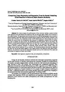
of using 200% over-sampling and 200% under-sampling was significantly better than the alternative of using the given data set on 57.6% of the 340 considered situations, while only on 3.2% of the cases sampling actually lead to a significantly worst model. The results also reveal that a slightly better outcome is obtained by the SmoteR approaches with respect to the alternative of simply under-sampling the most frequent values. Figure 1 shows the best scores obtained with any of the sampling and nosampling variants that were considered for each of the 17 data sets. As it can be seen, with few exceptions it is clear that the best score is obtained with some sampling variant. As expected the advantages decrease as the score of the baseline no-sampling approach increases, as it is more difficult to improve on results that are already good. Moreover, we should also mention that in our experiments we have considered only a few of the possible parameter variants of the two sampling approaches (4 in SmoteR and 2 with under-sampling).

F1 of Best Sampling and Best No−sampling ●

Sampling No−Sampling

0.8

●

●

●

0.6 0.4

F−1 Score

● ●

●

●

●

●

● ●

●

●

●

●

●

maxTorque

fuelCons

boston

cpuSm

availPwr

bank8FM

dElev

dAiler

Accel

Abalone

a7

a6

a5

a4

a3

a2

a1

0.2

●

Fig. 1: Best Scores obtained with sampling and no-sampling.

5

Conclusions

This paper has presented a general approach to tackle the problem of forecasting rare extreme values of a continuous target variable using standard regression tools. The key advantage of the described sampling approaches is their simplicity. They allow the use of standard out-of-the-box regression tools on these particular regression tasks by simply manipulating the available training data. The key contributions of this paper are : i) showing that sampling approaches can be successfully applied to this type of regression tasks; and ii) adapting one of the most successful sampling methods (Smote ) to regression tasks. The large set of experiments we have carried out on a diverse set of problems and using rather different learning algorithms, highlights the advantages of our

proposals when compared to the alternative of simply applying the algorithms to the available data sets. Acknowledgements This work is part-funded by the ERDF - European Regional Development Fund through the COMPETE Programme (operational programme for competitiveness), by the Portuguese Funds through the FCT (Portuguese Foundation for Science and Technology) within project FCOMP - 01-0124-FEDER-022701.

References 1. Domingos, P.: Metacost: A general method for making classifiers cost-sensitive. In: KDD’99: Proceedings of the 5th International Conference on Knowledge Discovery and Data Mining, ACM Press (1999) 155–164 2. Elkan, C.: The foundations of cost-sensitive learning. In: IJCAI’01: Proc. of 17th Int. Joint Conf. of Artificial Intelligence. Volume 1., Morgan Kaufmann Publishers (2001) 973–978 3. Zadrozny, B.: One-benefit learning: cost-sensitive learning with restricted cost information. In: UBDM’05: Proc. of the 1st Int. Workshop on Utility-Based Data Mining, ACM Press (2005) 53–58 4. Chawla, N.V.: Data mining for imbalanced datasets: An overview. In: The Data Mining and Knowledge Discovery Handbook. Springer (2005) 5. Zadrozny, B.: Policy mining: Learning decision policies from fixed sets of data. PhD thesis, University of California, San Diego (2003) 6. Ling, C., Sheng, V.: Cost-sensitive learning and the class imbalance problem. In: Encyclopedia of Machine Learning. Springer (2010) 7. Kubat, M., Matwin, S.: Addressing the curse of imbalanced training sets: Onesided selection. In: Proc. of the 14th Int. Conf. on Machine Learning, Morgan Kaufmann (1997) 179–186 8. Chawla, N.V., Bowyer, K.W., Hall, L.O., Kegelmeyer, W.P.: Smote: Synthetic minority over-sampling technique. JAIR 16 (2002) 321–357 9. Torgo, L., Ribeiro, R.P.: Precision and recall in regression. In: DS’09: 12th Int. Conf. on Discovery Science, Springer (2009) 332–346 10. Ribeiro, R.P.: Utility-based Regression. PhD thesis, Dep. Computer Science, Faculty of Sciences - University of Porto (2011) 11. Davis, J., Goadrich, M.: The relationship between precision-recall and roc curves. In: ICML’06: Proc. of the 23rd Int. Conf. on Machine Learning. ACM ICPS, ACM (2006) 233–240 12. Torgo, L., Ribeiro, R.P.: Utility-based regression. In: PKDD’07: Proc. of 11th European Conf. on Principles and Practice of Knowledge Discovery in Databases, Springer (2007) 597–604 13. Milborrow, S.: earth: Multivariate Adaptive Regression Spline Models. Derived from mda:mars by Trevor Hastie and Rob Tibshirani. (2012) 14. Dimitriadou, E., Hornik, K., Leisch, F., Meyer, D., Weingessel, A.: e1071: Misc Functions of the Department of Statistics (e1071), TU Wien. (2011) 15. Liaw, A., Wiener, M.: Classification and regression by randomforest. R News 2(3) (2002) 18–22