SNEE: A Query Processor for Wireless Sensor Networks - School of ...

Distributed and Parallel Databases manuscript No. (will be inserted by the editor)

SNEE: A Query Processor for Wireless Sensor Networks Ixent Galpin · Christian Y. A. Brenninkmeijer · Alasdair J. G. Gray · Farhana Jabeen · Alvaro A. A. Fernandes · Norman W. Paton

November 10, 2010 :: 18:31

Abstract A wireless sensor network (WSN) can be construed as an intelligent, large-scale device for observing and measuring properties of the physical world. In recent years, the database research community has championed the view that if we construe a WSN as a database (i.e., if a significant aspect of its intelligent behaviour is that it can execute declaratively-expressed queries), then one can achieve a significant reduction in the cost of engineering the software that implements a data collection program for the WSN while still achieving, through query optimization, very favourable cost:benefit ratios. This paper describes a query processing framework for WSNs that meets many desiderata associated with the view of WSN as databases. The framework is presented in the form of compiler/optimizer, called SNEE, for a continuous declarative query language over sensed data streams, called SNEEql. SNEEql can be shown to meet the expressiveness requirements of a large class of applications. SNEE can be shown to generate effective and efficient query evaluation plans. More specifically, the paper describes the following contributions: (1) a user-level syntax and physical algebra for SNEEql, an expressive continuous query language over WSNs; (2) example concrete algorithms for physical algebraic operators defined in such a way that the task of deriving memory, time and energy analytical cost-estimation models (CEMs) for them becomes straightforward by reduction to a structural traversal of the pseudocode; (3) CEMs for the concrete algorithms alluded to; (4) an architecture for the optimization of SNEEql queries, called SNEE, building on well-established distributed query processing components where possible, but making enhancements or refinements where necessary to accommodate the WSN context; (5) algorithms that instantiate the components in the SNEE architecture, thereby supporting integrated query planning that includes routing, placement and timing; and (6) an empirical performance evaluation of the resulting framework. Keywords Query Optimization · Wireless Sensor Networks · Distributed Query Processing · Query Languages · Continuous Queries · Cost Estimation Models

1 Introduction The sensor networks of interest to this paper are networks formed by wireless links between immobile nodes that are energy-constrained and possess both sensing and general-purpose computing capabilities. They offer the promise of direct, cost-effective access to observations and measurements of the physical world. In commercial settings, this can allow businesses to make their value-adding processes more responsive to physical phenomena. For example, in precision agriculture [12], such wireless sensor networks (WSNs) can inform finer-grained intervention tasks in response to changes in soil conditions for the purposes, say, of irrigation, or of pest control. In scientific settings, WSNs can act as intelligent data School of Computer Science, University of Manchester Oxford Road, Manchester M13 9PL, United Kingdom Tel.: +44 (0) 161 306 9280 Fax: +44 (0) 161 275 6204 E-mail: {ixent,brenninkmeijer,a.gray,jabeen,alvaro,norm}@cs.man.ac.uk

collection instruments that obtain readings for longer periods and over larger areas at a finer-grain in time and space than traditional data collection techniques are capable of achieving cost-effectively. For example, in the environmental sciences, they are becoming an essential enabling technology [34]. From the viewpoint of this paper, WSNs are taken to be a platform for distributed computing and, viewed as such, WSNs are unique in being constrained to an unprecedented extent compared to the predominant distributed computing platforms (e.g., the Web over the Internet). The constraint we focus on in this paper is that of depletable energy stocks for mote-level WSNs, i.e., WSNs whose nodes are low-cost, battery-powered devices with short-range radio components and very limited amounts of both volatile and persistent memory. This implies an optimization goal of conserving energy in order to extend the lifetime of a deployment. Given that wireless communication typically incurs a much greater energy cost than processing [49], it is generally accepted that processing data inside the WSN is likely to lead to longer lifetimes than simply sending that data unprocessed to a base station, where all the processing would then take place. We refer to these approaches as in-network processing and warehousing, respectively. The contributions reported pertain to the former approach. In the in-network processing approach, the question arises as to how much processing, roughly speaking, should take place inside the WSN. Broadly, one would like to instrument the WSN to only emit to the base station information of significant decision-making, or archival, value, i.e., information that is the outcome of processing (e.g., filtering, aggregating, cleaning, etc.). We note that, in scientific applications, many scientists prefer to pull all the raw data from the WSN for later analysis. However, we observe that, on the one hand, this option is not precluded by the in-network processing approach and, on the other, such a preference may not be viable as it may deplete energy resources prematurely. A trade-off that arises in the context of this paper is the one between the hardware and the software development costs associated with a WSN deployment. While hardware costs continue to fall, developing software for distributed platforms is in itself a complex endeavour, and the problem is far more acute in the case of mote-level WSNs due to their inherent limitations and constraints. It is likely, therefore, that, in the case of mote-level WSNs, bespoke software could incur such development costs as to offset or annul the savings made in purchasing the platform in the first place. This observation lies behind the challenge of reducing the cost of developing bespoke executables that enact energy-efficient data collection tasks over mote-level WSNs. A significant, and growing, literature (e.g., [7,28,8,44,62]) advocates that the declarative query paradigm, which has facilitated the uptake of traditional database technology, is likely to be effective in addressing the software development challenge posed by mote-level WSNs. In this case, the idea is, roughly speaking, to equate in-network processing with declarative query processing. In this way, the energy-conservation benefits of in-network processing are compounded with the cost-reduction benefits of declarative query processing. Thus, this research programme, referred to as the network-as-database approach [31], aims to develop sensor network query processors (SNQPs) that drastically reduce the need for bespoke development while ensuring sufficient low levels of energy consumption as to deliver deployments of great longevity. This paper presents, within this research context, a comprehensive account of a distributed query processing (DQP) framework for WSNs that accepts expressive declarative queries and generates query evaluation plans (QEPs) that perform well with respect to energy efficiency. The framework has been implemented as a compiler/optimizer, called SNEE [21,22], for a continuous declarative query language over sensed data streams, called SNEEql [10,11], and the code is available under the New BSD opensource licence at http://code.google.com/p/snee/1. SNEEql can be shown to meet the expressiveness requirements of a large class of applications. SNEE is distinctive in extending to SNQP the classical two-phase approach to DQP [40]. Our goal in doing so has been to explore the hypothesis that this approach allows for more expressive queries than other SNQP systems have supported to be efficiently evaluated over WSNs. The paper describes the following principal contributions: 1. a user-level syntax and physical algebra for SNEEql, an expressive continuous query language over WSNs;

1

Note that certain features described here may not yet have been made available in the latest stable release.

2

2. example concrete algorithms for physical algebraic operators defined in such a way that the task of deriving memory, time and energy analytical cost-estimation models (CEMs) for them becomes straightforward by reduction to a structural traversal of the pseudocode; 3. CEMs for the concrete algorithms alluded to; 4. an architecture for the optimization of SNEEql, called SNEE, building on well-established DQP components where possible, but making enhancements or refinements where necessary to accommodate the WSN context; 5. algorithms that instantiate the components in the SNEE architecture, thereby supporting integrated query planning that includes routing, placement and timing; and 6. an empirical performance evaluation of the resulting framework. Our account starts with a consideration, in Section 2, of the technical background and the research context for our contributions. Then, in Section 3, we briefly consider the functional and non-functional requirements that such a framework must support as elicited from the literature on WSN deployments and one detailed case study. Section 4 consists of a description of the SNEEql continuous declarative query language including a discussion of its syntax, its underlying logical and physical algebras, and of the analytical CEMs for energy, duration, and memory that are associated with the physical operators. Section 5 is devoted to a comprehensive description of the SNEE compiler/optimizer. We describe the functional decomposition of SNEE into a query compilation/optimization stack that extends its classical counterparts in novel ways. We also describe in detail the optimization strategies involved, we explain the crucial role of the analytical CEMs described in Section 4, and we conclude the section with a description of how SNEE uses code generation techniques to emit source code in nesC/TinyOS, the de facto standard software runtime language/libraries for mote-level WSNs [27,41]. Section 6 is dedicated to presenting experimental evidence that SNEE satisfies the most important non-functional requirements placed upon it for a large collection of SNEEql queries. Finally, in Section 7, we reflect on the contributions reported and we indicate the extensions and enhancements that we are currently pursuing.

2 Related Work 2.1 On Sensor Network Query Languages One of the motivations behind SNEEql was to provide more expressiveness than previous sensor network query languages, such as TinyQL [44], Cougar [18,62], and SNQL [8]. Our intention was to design a sensor network query language with expressiveness comparable to continuous query languages that have been proposed to query data streams over relatively unconstrained infrastructures compared to WSNs, e.g., [4,13,37]. To achieve this, we took CQL [4] as our starting point, primarily because it construes windows as resulting from type conversion of streams of tuples into streams of bags of tuples, which enables greater reuse of classical techniques at the level of the logical and physical algebras prior to query plan fragmentation and distribution. As a result, compared to existing sensor network query languages, SNEEql has a richer data model and a clearer data definition language (closer to Cougar’s and more convenient than TinyQL’s, in that the latter uses a universal relation approach to model WSN data). Furthermore, SNEEql has flexible (but not overwrought) window specifications comparable in expressiveness to those present in existing continuous query languages for stream query processors. SNEEql, like CQL, uses a window-based approach to provide uniform support for blocking operators (such as joins and aggregations). In contrast, TinyQL resorts to materialization points and only offers relatively limited support for blocking operators since it does not allow window specifications (other then for aggregates). On the other hand, TinyQL offers support for event specifications, which are, currently, unsupported in SNEEql. Finally, none of the other sensor network query languages in the literature has been described in as much detail as SNEEql (the closest being SNQL [8]). In Section 4, and in other publications [10,11,9] that complement this paper, we show that SNEEql can be assigned a formal syntax and semantics. 3

2.2 On Sensor Network Cost Estimation Models SNEEql language constructs can also be cast as a set of well-defined logical and physical algebraic operators. Such physical operators can be mapped to concrete algorithms for which we have derived memory, duration and energy CEMs (in the form of empirically-validated analytical expressions) that can guide decision making by query optimizers. It is generally recognized that CEMs play an important role in classical and distributed query optimization [15,26,50]. Their availability means that a QEP can be assessed, in isolation and in comparison to alternative QEPs, in terms of the extent to which it meets some non-functional property of QEPs (classically, the response time it delivers). Recently, the extension of query technology to data streams has once more highlighted the relevance of CEMs: [16] describes how they are used to inform the placement of a selection with respect to a join in a multiple query setting, and [61] proposes a rate-based approach to CEMs rather then the traditional cardinality-based one. The latest, and perhaps the most challenging, query optimization problem in which CEMs play a fundamental role is that of optimizing declarative queries for execution over WSNs [6,28]. Section 4 describes how empirically-validated CEMs for the space, time and energy consumed by a QEP over a WSN were methodically derived and validated for an expressive algebra for continuous queries over acquisitional sensor-data streams.

2.3 On Sensor Network Query Processing There have been many proposals for SNQPs (including [7,28,8,44,62]). Surprisingly, none have fully described an approach to query optimization founded on a classical DQP architecture. Cougar papers [28] propose this idea but no publication describes its realization. SNQL [8] follows the idea through but no precise description (as provided by our algorithms) of the decision-making process has been published. Indeed, few publications provide systematic descriptions of complete query optimization architectures for WSN query processors: the most comprehensive description found was for TinyDB [44], in which optimization is limited to operator reordering and the use of CEMs to determine an appropriate acquisition rate given a user-specified lifetime. Arguably as a result of this, WSN-as-database proposals have tended to limit the expressiveness of the query language. For example, TinyDB focuses on aggregation and provides limited support for joins. In many cases, assumptions are made that constrain the generality of the approach (e.g., Presto [24] focuses on storage-rich networks). There has also been a tendency to address the optimization problem in a piecewise manner. For example, the trade-off between energy consumption and time-to-delivery is studied in Wave Scheduling [59]; efficient and robust aggregation is the focus of several publications [42,46,58]; Bonfils [6] proposes a costbased approach to adaptively placing a join which operates over distributed streams; Zadorozhny [64] uses an algebraic approach to generate schedules for the transmission of data in order to maximize the number of concurrent communications. However, these individual results are rarely presented as part of a fully-characterized optimization and evaluation infrastructure, giving rise to a situation in which research at the architecture level seems less well developed than that of techniques that might ultimately be applied within such query processing architectures. In Section 5, and in other publications [21,22] that complement this paper, we have aimed to provide a comprehensive, top-to-bottom approach to the optimization problem for expressive declarative continuous queries over potentially heterogeneous WSNs. In comparison with past proposals, ours is broader, in that there are fewer compromises with respect to generality and expressiveness, and more holistic, in that it provides a top-to-bottom decomposition of the decision-making steps required to optimize a declarative query into a QEP. Furthermore, much research in the area has also focussed on energy preservation by the use of probabilistic techniques that involve prediction and/or giving approximate answers. For example, BBQ [19] addresses the trade-off between acquiring data often and the cost of doing so. Other related approaches include the Ken approach [17] and PAQ [60], in which only tuples that do not conform a statistical model are transmitted to the gateway node. Proposals have also been made for joins in which the accuracy of results are traded for the amount of data transmitted (e.g., [63]). Currently the SNEE physical operators proposed in this paper work do not drop tuples, and aim to give complete answers. However, such approaches are not precluded by the SNEE architecture described in this paper, and could be implemented by the incorporation of additional physical operators (with associated CEMs). 4

3 WSN Application Requirements When environmental scientists use WSNs, it is often with a view to collecting time series. Time series produced by live sensing devices are data streams [29]. Many of the papers on stream systems and their query languages [1,4,14,33,51] are focused on how they were implemented, without detailed motivation as to why the included features are required. This section examines user needs using three example WSN deployments described in the literature. Our account of the example deployments has been slightly adapted to demonstrate what could potentially be done and not just what was described as having actually been done. Note that in this section, we use examples to introduce syntactic forms and constructs. A more formal account is provided in Section 4. Note also that the current implementation of SNEE/SNEEql does not yet support all the constructs we have identified as useful, although we have described their semantics in detail in [10]. In particular, in [10] we have shown how SNEEql has a uniform semantics over any combination of push streams, pull streams and stored extents, a feature that, we postulate, expands the applicability of continuous query processing in a significant way.

3.1 Example Deployments We will motivate the features and constructs available in SNEEql by reference to three example deployments, as follows. The first deployment, as described in [47], was at Crowden Great Brook, a small stream in the UK Peak District. The purpose of the deployment was to assess the hydro-dynamics of surface water drainage. With that goal, a team of environmental scientists deployed a small WSN in the region surrounding a stretch of the brook. The second deployment, as described in [5,12], was on the Okanagan Valley, a wine-producing region in British Columbia, Canada. The purpose of the deployment was to carry out a precision agriculture study in order to find areas where WSNs can deliver valuable information and provide a return on investment. The third deployment, as described in [45,55, 56], was at Great Duck Island, in the Gulf of Maine, which is home to the largest petrel colony in the eastern coast of the USA. WSN technology was used to study the nesting patterns of the petrels with respect to the weather conditions. We note that the deployments described here all involve sensor nodes whose location is (expected to be) fixed as data is gathered. The current version of SNEE is unsuitable for applications where the nodes are mobile, e.g., as described in Zebranet [65]. The three example deployments provide compelling evidence for the usefulness of the classical operations (viz., selection, projection, join and aggregation) on logical extents that are classically expressible by declarative query languages. Of course, a WSN is a source of acquisitional data streams (i.e., streams whose items do not enter the system at unknown arrival rates but rather according to a user-specified acquisition, or sampling, rate) [43]. This means that queries over WSNs are continuous (and, more specifically, reactively-reevaluated) queries [29]. As is well known [29], in this case, blocking operations (such as join, sort and various forms of aggregation) only have a well-defined semantics over a bounded subset of the stream, i.e., over so-called windows over the stream. We now show how these query language constructs (i.e., logical extents, possibly with windows defined on them, over physical acquisitional streams to which one can apply selection, projection, join and aggregations) capture most of the functionality targeted by the example deployments above. For example, in the Crowden Great Brook deployment, the scientists involved were mostly concerned with generating a time series of robust measurements because their research aims were mostly speculative, in the sense of not being driven by a hypothesis (i.e., the scientists’ main concern was to obtain representative data for out-of-network exploration unframed by any preconceived assumptions as to the behaviour of the underlying physical phenomena). The data of interest can therefore be easily characterized as follows: every two hours, for each node id, take the per-attribute average of the values observed in that node (e.g., moisture, temp) over the last two hours, and timestamp it with the latest time value available in the node. Fig. 1(a) shows how SNEEql can capture the data of interest. The fact that aggregation is pushed into the WSN means that there is a certain amount of data reduction, thereby prolonging the lifetime relative to the alternative of warehousing all the observed data back at base. However, because aggregation is irreversible, this approach does mean that some observations are no longer directly available. If the scientists wanted to retrieve all the measurements obtained, a SNEEql SELECT-star query could be issued. 5

SELECT R.id, MAX(R.time), AVG(R.moisture), AVG(R.temp) FROM River R [FROM NOW TO NOW-2 HOURS] GROUP BY R.id (a) Crowden Great Brook

SELECT FROM WHERE

MAX(V.time) AS time, COUNT(V.moisture) AS drySites Vineyard[NOW] V V.moisture < 20;

(b) Okanagan Valley

SELECT FROM WHERE

B.time, B.id, B.temp, W.temp Burrow[NOW] B, Weather[NOW] W B.temp > W.temp AND B.id = W.id;

(c) Great Duck Island Fig. 1 Queries for Example Deployments

In the case of the Okanagan Valley deployment, one information of interest might be how many sites are dry (i.e., have a moisture value less than a given threshold). Fig. 1(b) shows how this requirement can be expressed in SNEEql. Note the use of selection and projection as two strategies for data reduction that preserve all observations of interest. Projection prevents the transducers sensing for physical quantities that were not relevant for the study, e.g., temperature, from firing in the first place. Savings were also made by using selection to remove readings which are outside the range of interest. Users will often be interested in associating values from different sources of data (e.g., comparing them). Since different sources are represented as different logical extents, such comparisons can often be captured using joins. This often requires, in the case of queries over streams, the use of windows. For example, in the Great Duck Island deployment, data collected from Burrow sites and Weather sites could be associated by constructing tuples in which the temperature inside the burrow is higher than in the nearby weather site. The SNEEql query in Fig. 1(c) reports back this information. For each point in time for which data is collected, this query creates windows over both source streams containing only the values measured at that point in time. It then joins the contents of the windows (using the equality predicate in the WHERE clause), filters out the tuples that do not satisfy the selection predicate, and projects out the attributes listed in the SELECT clause. It is also often useful to take into account the natural delay in some temporally and spatially extended phenomena, e.g., one could have the temperature in burrows be compared with that of a weather station a few minutes previously depending on the distance between the sites and, say, the direction of the prevailing weather fronts. The precision agriculture deployment also illustrates well how joins can be used to detect associations between observations that trigger actions on the part of the users. For example, an indication as to whether an area may be in need of watering may be detected by associating the humidity readings at one period with the humidity readings at the immediately preceding period, i.e., consistent falls in humidity at a significant rate can be taken as an indication that watering may be required. Note that, here too, the ability to compute and compare moving averages is useful.

3.2 A Running Example In order to describe in more detail a greater range of issues and features, we will use a running example that is closely inspired by the Crowden Great Brook deployment but is not precisely accurate with respect to its description in the literature. Assume that we are investigating a model of surface water drainage in the Crowden Great Brook area of the Peak District in the UK. The site is hilly, with some areas covered with peat. Water drains into a valley at the bottom of which flows a brook.

River: (id:int, time:int, rain:int, depth:int) Hilltop: (id:int, time:int, rain:int) Fig. 2 Example Logical Schemas.

6

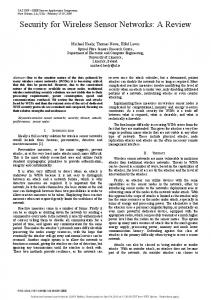
Assume that a WSN with ten nodes numbered {0, 1, 2, 3, 4, 5, 6, 7, 8, 9} has been deployed to study the interaction of rainfall and river depth. Let River be one logical extent with sources at nodes 5, 6, 7, 9 and let Hilltop be another logical extent with a single source at node 4, with schemas as shown in Fig. 2. Assume that radio connectivity is such that the following edges denote the pairs of nodes that can communicate with each other: {0:1, 0:2, 2:4, 1:4,1:3, 3:6, 3:5, 4:5, 5:7, 4:8, 7:8, 7:9, 8:9}, and let the delivery point be node 0, as depicted in Fig. 3. To illustrate the expressiveness of (the publicly-available implementation of) SNEEql using this scenario as an example, consider the queries in Fig. 4. The query in Fig. 4(a) returns a stream of tuples (more precisely, pairs of time and depth values) that are filtered from the stream of sensor readings logically denoted by River, emitting into the output only those that have a measured depth greater than 10. Using window specifications, one can perform aggregations over specific time intervals or over certain samples. The query in Fig. 4(b) is a variant on Fig. 4(a). Rather than projecting out, the measured depth, it projects the average depth over the last 10 tuples in the stream. Windows also allow for joins to be expressed in the usual manner. The query in Fig. 4(c) joins tuples from the River and Hilltop extents provided that the rain measured now in the river is less than that measured on the hilltop 15 minutes ago, and provided that that rain measurement was above 5. The query in Fig. 4(d) illustrates support for subqueries. It is a variant on Fig. 4(a) in which tuples are only emitted into the result stream if the river depth now is larger than the average depth over the last seven days. The next section describes the SNEEql language more formally. Section 5 describes in detail how SNEE compiles SNEEql queries into optimized QEPs.

Fig. 3 The Example Deployment. Black circles denote sources for the River extent, and the white circle is a source for the Hilltop extent.

4 The SNEEql Continuous Declarative Query Language This section describes the SNEEql continuous query language. We begin, in Section 4.1, by describing the underlying type system. In Section 4.2 we then briefly describe the main syntactic constructs of the language. We show with an example how the surface forms are translated (by the standard procedure for SQL-like languages) into a logical-algebraic form (Section 4.3). We describe the physical algebra that we have developed for SNEEql (Section 4.4) and exemplify the concrete algorithms we have used to instantiate the physical operators (Section 4.5). Finally, in Section 4.6, we give examples of how we have derived CEMs for memory, duration and energy from the algorithmic instantiation of the operators. 7

SELECT FROM WHERE

R.time, R.depth River R R.depth > 10;

SELECT FROM WHERE

(a) A Select-Project Query

SELECT FROM WHERE

R.time, AVG(R.depth) River [RANGE 10 ROWS SLIDE 10 ROWS] R R.depth > 10;

(b) A Window-Based Aggregation Query.

R.time, H.rain, R.depth River [NOW] R, Hilltop [AT NOW-15 MINUTES] H H.rain > 5 AND R.rain < H.rain (c) A Window-Based Join Query.

SELECT FROM

WHERE

R1.id, R1.time, R1.depth River [NOW] R1, (SELECT AVG(R2.depth) as avgDepth FROM River [NOW-7 DAYS] R2) LastWeek R1.depth > LastWeek.avgDepth (d) Query/Subquery Correlations.

Fig. 4 Example SNEEql queries.

4.1 SNEEql Data Model The primitive types are integer, float, string and time. The compound types are tuple and tagged tuple. A tuple type consists of a set of typed attributes, a1:t1 , . . . , an:tn , where each ai is an attribute name and each ti is a primitive type. A tagged tuple type is a tuple type including two distinguished attributes: one named tick of type integer, and another named index of type integer. Values of type tick are drawn from a system-wide ordinal domain, those of type index are ordered inside the collection in which they appear. A tick value denotes the timestamp in which a tagged tuple was created, an index value denotes its position in a sequence where it was placed. The collection types are window and stream. A window type is a pair whose first element is a distinguished attribute, named tick, of type integer, denoting the timestamp in which the window was created, and whose second element is of type bag of tuples of the same tuple type. A stream is a potentially infinite, append-only sequence of values of the same tagged tuple or window type. Note that tick and index are implicitly-defined attributes of tagged tuples, as is tick for windows. In [10], we have described in detail how SNEEql can associate to its logical extents, physical extents that can be pulled (or sensed), pushed or stored. In this paper, however, we confine ourselves to sensed extents in order to keep as close as possible to the publicly-released version of the SNEE framework. Sensed extents are pull-based, i.e., associated with a declared acquisition rate (one tuple every fifteen minutes per acquisition site, in our running example), and for this reason can also be referred to as acquisitional. Streamed extents are push-based, i.e., associated with an unknown, potentially variable, arrival rate. From the viewpoint of continuous SNEEql queries, both sensed and pushed extents are streams of tagged tuples, whereas stored extents are streams of windows. As an example SNEEql schema, consider the deployment described above and note that its logical schema can be specified as in Fig. 2.

4.2 SNEEql Syntax This section introduces the main kinds of SNEEql queries, viz., stream queries and window queries2 . Stream queries are of the form SELECT a1 . . . an FROM s WHERE p

(1)

where a1 . . . an is a projection list, s denotes a stream of tagged tuples (i.e., the name of an extent, or a subquery, of type stream of tuple), and p is a predicate. There are semantic restrictions on stream queries, as follows: firstly, the FROM clause must reference a single stream because cross product is not 2

An overview of the formal semantics of SNEEql queries is available in [10], and detailed, exhaustive accounts of both their formal syntax and their formal semantics are given in [9].

8

well defined over infinite collections, and, secondly, the projection list elements ai cannot involve the application of aggregation functions on values from s. Evaluating a stream query yields a stream of tagged tuples. Window queries are of the form SELECT a1 . . . an FROM w1 . . . wm WHERE p

(2)

where a1 . . . an is a projection list, w1 . . . wm is a list of window definitions, and p is a predicate. Window queries can also contain GROUP BY and HAVING clauses in the standard way. Evaluating a window query yields a stream of windows. Each wi in the FROM clause specifies a window on the name of an extent, or a subquery, of type stream of tuple, as follows. A window on a stream is of the form s[FROM t1 TO t2 SLIDE int unit]

(3)

where s denotes a stream of tagged tuples (i.e., the name of an extent, or a subquery, of type stream of tuple), and both ti are either of the form NOW or NOW − int unit, where NOW denotes the current tick or index, int is a positive integer, and unit ∈ {SECONDS, MINUTES, HOURS, DAYS, ROWS}. The FROM and TO parameters define a window that selects all tuples in s in the range relative to when the window is created, while the SLIDE parameter determines how often a new window is created. When t1 = t2 , the shorthands AT t1 and AT t1 − int can be used instead of a FROM/TO pair. The shorthand RANGE d is used to denote an interval from NOW − d to NOW. Also, when t1 = t2 = NOW, the shorthand NOW can be used can be used instead of a FROM/TO pair. Finally, the result of a SNEEql window query can be converted into a stream using the CQL-inspired type-conversion functions RSTREAM (which emits all tuples in the window), ISTREAM (which emits all tuples that have become part of the window since the last evaluation) and DSTREAM (which emits all tuples that have ceased to be part of the window since the last evaluation) [4]. Given the SNEEql schema in Fig. 2, Fig. 5 shows the SNEEql query whose compilation and optimization we will describe in detail in Section 5. The process of compiling and optimizing a SNEEql query is informed by quality-of-service (QoS) expectations. In the current implementation of SNEE, two QoS expectations can be provided (as invocation-time parameters), viz., the acquisition (or sampling) rate, which we denote by α, and the maximum delivery time, which we denote by δ. The acquisition rate determines how often the QEP causes data to be sensed. The delivery time denotes the amount of time that passes between a value being sensed and it being delivered at the root of the QEP.

4.3 Logical Algebra The logical algebra associated with SNEEql is an extension of a classical select-project-join-aggregation relational algebra. The extensions consist of, firstly, explicit acquisition and delivery operators that play the role of generating an acquisitional stream of tuples and delivering results, and, secondly, type conversion operators that generate a stream of windows from a stream of tuples, or vice-versa. The translation of a SNEEql query into its logical-algebraic form (LAF) is based on the standard translation [25] of a SQL-like query into a select-project-product algebraic expression to which optimizers then apply rule-based rewriting strategies. To recall, the procedure consists of creating a Cartesian product of all the extents in the FROM clause, applying the predicate expression in the WHERE clause to that product, and, finally, from the tuples thus obtained retaining only those attributes defined by the expressions in the SELECT clause. Some examples of the extensions required in the case of SNEEql for RSTREAM FROM WHERE AND

SELECT River.time, Hilltop.rain, River.depth River[NOW], Hilltop[AT NOW-15 MINUTES] Hilltop.rain > 5 River.rain < Hilltop.rain;

QoS Expectations: h Acquisition Rate = 15 Minutes, Delivery Time = 24 Hours i Fig. 5 The Example Query and Quality-of-Service Expectations in SNEEql

9

RSTREAM w ⇒ RSTREAM (w ′ ) (a) RSTREAM translation. SELECT a1 . . . an FROM w1 . . . wm WHERE p ⇒ PROJECT[a1 . . . an ] ( SELECT[p] ( ′ ) )) CROSS PRODUCT (w1′ ), . . ., (wm (b) Window query. s[AT t timeU nit] ⇒ TIME WINDOW[convert(t,timeU nit),convert(t,timeU nit),α] ( SP ACQUIRE (*, true, s, α)) (c) Window over an acquisitional stream. Fig. 6 Example rules for translating SNEEql syntax to logical algebra.

the query in Fig.5 are captured by translation rules presented in Fig. 6. Fig. 6(a) presents the rule for translating the RSTREAM clause, used to convert a stream of windows w into a stream of tuples. The result is the RSTREAM operator with w′ (the translation of w) as an input. The subquery within the RSTREAM in Fig. 5 has the form of a window query (as defined in Section 4.2) and is translated according to the rule in Fig. 6(b). The time window in Fig. 5 is translated using the rule in Fig. 6(c), using the convert function to ensure that the time interval is expressed in consistent units in the algebra. α denotes the acquisition rate specified in the QoS. The initial LAF is rewritten using standard equivalence-preserving transformations used in classical query processing, including pushing down projections and selections, and collapsing a select and a Cartesian product into a join [25]. In addition, transformations similar to those in CQL such as pushing a selection and projection below a time window are performed [3]. If possible, selections are pushed into the acquisition operator. In [10,9], the translation and rewriting of a SNEEql query is explained in detail. Fig. 7 shows the translation of the SNEEql query in Fig. 5 into the LAF that results from this standard translation3 . Definitions of the physical-algebraic versions of the operators are given in Table 1.

DELIVER

RSTREAM

JOIN River.rain < Hilltop.rain

TIME_WINDOW [t−15, t−15, 15]

SP_ACQUIRE [time, rain, depth] true River EVERY 15 min

SP_ACQUIRE [time, rain] rain > 5 Hilltop EVERY 15 min

Fig. 7 The Example Query in Logical-Algebraic Form

10

Stream-to-Stream Operators ProjList , Take a reading every AcqInt from sensors in AttrList and apply SELECT[PredExpr ] and PROJECT[ProjList ] in that order on the resulting tuple. DELIVER[ ](S) : S Deliver the query results. Stream-to-Window Operators TIME WINDOW[startTime, endTime, slide](S) : Define a time-based window on S from startTime W to endTime inclusive and re-evaluate every slide time units. ROW WINDOW[startRow, endRow , slide](S) : Define a tuple-based window on S from startRow W to endRow inclusive and re-evaluate every slide rows. Window-to-Stream Operators RSTREAM[ ](W ) : S Emit onto S all the tuples in W . ISTREAM[ ](W ) : S Emit onto S the newly-inserted tuples in W since the previous window evaluation. DSTREAM[ ](W ) : S Emit onto S the newly-deleted tuples in W since the previous window evaluation. Window-to-Window Operators NL JOIN[ProjList, PredExpr ](W ,W ) : W Using the nested-loop join algorithm, emit onto the output the concatenation of each tuple from the left to each tuple from the right input (keeping only the attributes in ProjList ) if it satisfies PredExpr . AGGR INIT[AggrFunction, ProjList ](W ) : W Initialize incremental aggregation for attributes in ProjList for type of aggregation specified by AggrFunction. AGGR MERGE[AggrFunction, ProjList](W ) : W Merge into the partial result the values from input for attributes in ProjList for type of aggregation specified by AggrFunction. AGGR EVAL[AggrFunction, ProjList ](W ) : W Emit into the output the final result of incrementally aggregating the attributes in ProjList for type of aggregation specified by AggrFunction. Any-to-Same-as-Input-Type Operators SELECT[PredExpr ](X): X Emit onto the output every tuple from the input that satisfies PredExpr . PROJECT[ProjList ] (X): X Emit onto the output a tuple formed with the atributes from the input tuple that occur in ProjList . Exchange Operators TRANSMIT[ ](X):X Pack input tuples into blocks up to the maximum packet size and send them over radio. RECEIVE[ ](X):X Receive blocks of up to the maximum packet size, unpack the tuples and emit them. SP ACQUIRE[AttrList, AcqInt ](S) : S

PredExpr ,

LocSen.

LocSen.

AttrSen.

AttrSen.

AttrSen. AttrSen.

Table 1 SNEEql Physical Algebra.

4.4 Physical Algebra Table 1 shows a comprehensive sample of the physical algebra underlying SNEE. It describes the operators, grouped by their respective input-to-output collection types. A signature has the form OPERATOR NAME[Parameters](InputArgumentTypes):OutputArgumentTypes, where the argument types are denoted S and W , for stream and window, resp., and X indicates either of the types given. Note that operators can be flagged as LocSen, denoting it to be location-sensitive or as AttrSen, denoting it to be attribute-sensitive. These are semantic properties of the operators and constrain the set of candidate nodes that the optimizer can assign them to when deciding where such operators should execute. Roughly speaking, a location-sensitive operator (e.g., any SP ACQUIRE and any DELIVER4 ) has a user-specified site in which it can execute by virtue of the WSN deployment (e.g., in our example, the DELIVER operator can only execute at node 0, which is the delivery point, and the 3 Note that the base time units in the algebra are milliseconds. To fifteen minutes, there correspond 900,000 milliseconds, but we use fifteen minutes (without unit) for legibility. 4 Note that SP ACQUIRE combines three logical operators (viz., SELECT, PROJECT and ACQUIRE) into a single physical operator, and that the same happens with DELIVER and RSTREAM.

11

DELIVER

RSTREAM

NL_JOIN River.rain < Hilltop.rain

TIME_WINDOW [t−15, t−15, 15]

SP_ACQUIRE [time, rain, depth] true River EVERY 15 min

SP_ACQUIRE [time, rain] rain > 5 Hilltop EVERY 15 min

Fig. 8 Example Query: The Physical-Algebraic Form Assigned by SNEE

SP ACQUIRE operators can only execute at nodes 5, 6, 7, 9, in the case of the River extent, and at node 4, in the case of the Hilltop extent). Again, roughly speaking, an attribute-sensitive operator must be placed at a node through which tuples from all the appropriate horizontal partitions (on the relevant attribute) flow. For example, NL JOIN is attribute sensitive, i.e., it must be placed at a node through which input tuples with different origins flow. We return to these notions and their consequences in the next section. Note, finally, that since SNEE is a DQP framework, we make use of Volcano-inspired EXCHANGE operators [32] which, in our case, encapsulate physical communication capabilities. This is manifest in the physical-algebraic form (PAF) in the TRANSMIT and RECEIVE operators shown in Fig. 17, since EXCHANGE operators are two-part operators, consisting of a producer and a consumer component in the source and target sites, respectively. Fig. 8 is the tree representation of the PAF corresponding to the LAF in Fig. 7. We now show how the operations in the SNEEql physical algebra can be expressed as concrete algorithms at a level in which it becomes possible to structurally derive CEMs for memory, duration and energy for them.

4.5 Concrete Algorithms Due to lack of space, we illustrate our methodology with the SP ACQUIRE and TRANSMIT physical operators because these illustrate representative data processing and movement capabilities. We have applied the same methodology to all other operators in the physical algebra [9]. We define the SP ACQUIRE and TRANSMIT operators in the remainder of this section, and the CEMs derived for them in Section 4.6. Broadly, the methodology is as follows: (1) we define, in pseudocode, the processing logic of an operator that gets executed at an evaluation episode (i.e., the equivalent to a getNext() in a classical physical operator that is designed for pipelined execution; (2) we declare, in the pseudocode, the state kept by the operator to support the processing logic in (1); (3) we fairly directly derive from (2) a CEM for memory; (4) we derive from the algorithmic structure of the operator (as revealed in the pseudocode) a CEM for duration in the classical way, i.e., we take into account the most expensive steps, using multipliers when the step is iterated; and, finally, (5) we derive from the CEM for duration obtained in (4) a CEM for energy by multiplying each addend in the former by the corresponding unit cost in energy. We have validated the analytical cost models thus obtained by means of an extensive empirical study, as reported in [11,9]. The main notational conventions we use are as follows: we set keywords in Roman bold, comments and variable identifiers (such as i and j ) in italic, the identifiers of auxiliary, lower-level functions in small lower-case sans-serif, and SYSTEM-WIDE PARAMETERS in upper-case sans-serif font. The SP ACQUIRE physical operator (in Fig. 9) performs three operations from the corresponding logical algebra: it acquires a tuple of sensed data as defined by AttrList, then it performs a select 12

SP 1 2 3 4 5 6 7 8 9 10 11 12 13 14 15 16

ACQUIRE[AttrList, PredExpr , ProjList , ](tick ) dependencies  CPU: on; Sensor Board: on; Radio: off state sensedValues: array of float size length(AttrList ) result: array of float size length(ProjList )+1 i : int  ACQUIRE for i =1 to length(AttrList ): do sensedValues[i ] ← sense(typeof(AttrList [i ]))  SELECT if apply(PredExpr , sensedValues ): then  PROJECT result [0] ← tick for j =1 to length(ProjList ): do result [j ] ← apply(ProjList [j ], sensedValues ) return bagof(result ) else return bagof([ ])

Fig. 9 Pseudocode for SP ACQUIRE. TRANSMIT[ ](tick, child ) 1 dependencies  CPU: on; Sensor Board: off; Radio: on 2 state 3 resultsFromChild  a pointer to 4 block : array of tuple size ⌊ (MAX PACKET SIZE/sizeof(tuple)) ⌋ 5 packet: array of byte size MAX PACKET SIZE 6 i : int 7 resultsFromChild ← child.getNext(tick ): 8 i ←1 9 for t ∈ resultsFromChild : 10 do block [i ] ← t 11 i ← i +1 12 if i = length(block )+1: 13 then  we have a full block 14 packet ← convert(block ) 15 send(packet ,sizeof(block )) 16 i ←1 17 if i > 1: 18 then  the last block is not full, so pad it 19 for j=i to length(block ): 20 do block [j] = NULL 21 packet ← convert(block ) 22 send(packet ,sizeof(block )) Fig. 10 Pseudocode for TRANSMIT.

operation using P redExpr, and finally, on those tuples that satisfied the selection condition, it performs a project operation using P rojList. The TRANSMIT physical operator (in Fig. 10) obtains (a pointer to) the results from its child operator and then packs tuples into a block containing as many tuples as will fit given the system-wide MAX PACKET SIZE parameter, making sure that the last block is padded with null bytes if it is not full.

4.6 Derived Cost Estimation Models In this section, we show how the style of pseudocode used in Section 4.5 can be built upon with a view to deriving memory, duration and energy CEMs for the corresponding operator (see [11] for parameter values corresponding to the sensors we have used in validating the CEMs). Note that P when expressing an aggregation, e.g., sum over a set of values V = {v1 , . . . , vn }, rather than write v∈V (v), we write sum{v | v ∈ V }. Finally, we note that the energy CEMs contain cross-references to the corresponding duration CEMs for the purposes of abbreviation only. Such references point to an addend in one equation in the duration CEM and should be interpreted in terms of textual substitution, i.e., textually replacing the reference with the expression it is a reference to yields the non-abbreviated form of the CEM. The CEMs for SP ACQUIRE are collected in Fig. 11, those for TRANSMIT in Fig. 12. 13

MSP ACQUIRE[AttrList, ,P rojList, MSP A OVERHEAD + sizeof(tick) +

](tick)

=

(4)

sum{sizeof(s) | s ∈ AttrList} + sum{sizeof(a) | a ∈ P rojList} DSP ACQUIRE[AttrList,P redExpr,P rojList, DSP A OVERHEAD +

](

),sensedV alues

=

(5) (6)

(sum{DSENSE(typeof(s)) | s ∈ AttrList}) +

(7)

(DAPPLY (A P, sensedV alues) ∗ count{p | p ∈ P redExpr ∧ atomic(p)}) +

(8)

(sum{DAPPLY (A E, sensedV alues) ∗ count{e | a ∈ P rojList ∧ e ∈ a ∧ atomic(e)})

(9)

ESP ACQUIRE[AttrList,P redExpr,P rojList, (ESENSE ∗ Addend[7].Eq(5)) +

](

)

=

(10)

EPROCESS ∗ (Addend[6].Eq(5) + Addend[8].Eq(5) + Addend.[9].Eq(5) ∗ sel(P redExpr)) Fig. 11 CEMs for SP ACQUIRE. MTRANSMIT[ ](tick,child) = MTRANS

OVERHEAD

(11)

+ sizeof(pointer) +

(sizeof(tuple) ∗ ⌊(MAX PACKET SIZE/sizeof(tuple))⌋) + MAX PACKET SIZE + sizeof(i) DTRANSMIT[ ](tick,child) = DTRANS

OVERHEAD +

(Dchild.getNext(tick) ) + ( (DRX

OVERHEAD

+

DTX

OVERHEAD

+

(DTX

BYTE

(12) (13) (14) (15) (16)

∗ sizeof(block))) ∗

(17)

⌈count{t ∈ resultsF romChild}/length(block)⌉) ETRANSMIT[ ](tick,child) =

(18)

(EPROCESS ∗ Addend[13].Eq(12)) + (EPROCESS ∗ Addend[14].Eq(12)) + (( ((EPROCESS + ERX ) ∗ Addend[15].Eq(12)) + ((EIDLE + ETX ) ∗ Addend[16].Eq(12)) + ((EIDLE + ETX ) ∗ Addend[17].Eq(12))) ∗ ⌈count{t ∈ resultsF romChild}/length(block)⌉) Fig. 12 CEMs for TRANSMIT.

Since the pseudocode declares the state kept in support of its processing logic, deriving a CEM for memory is tantamount to writing a summation in which each addend is the result of applying a primitive like sizeof to each scalar variable and summing the scalar elements in collection variables. This process is illustrated in Eq. (4) in Fig. 11, bearing Fig. 9 in mind. The derivation of a CEM for duration is similarly straightforward. The only additional concerns are: (a) to focus on steps which use processing more intensively (disregarding, e.g., atomic steps that do not involve calls to potentially expensive functions), and (b) to formulate the expressions that act as multiplicands on the processing blocks that are iterated over and that quantify the number of passes in the iteration. This process is illustrated in Eq. (5) in Fig. 11, bearing Fig. 9 in mind. Some parameters of interest in Eq. (5) are, DSENSE(typeof(s)) , the time it takes to sense a value of a given type, A P and A E, the time it takes to evaluate an atomic Boolean and an atomic arithmetic expression, respectively. Finally, note that, for complex predicate and arithmetic expressions, we abstract the workload involved in terms of the number of atomic expressions the expression tree contains. The derivation of a CEM for energy, given the corresponding duration CEM, is also straightforward. If we bear in mind that sensor nodes consume different amounts of unit energy for sensing, processing, receiving and transmitting, then the derivation of an energy CEM from a duration CEM essentially amounts to (1) classifying each addend in the duration CEM by the types of energy being spent in its duration, and (2) multiplying the durations thus obtained by the corresponding unit energy cost. This process is illustrated in Eq. (10) in Fig. 11, bearing Fig. 9 in mind. In SP ACQUIRE, there is no use of 14

radio, so the unit energy costs involved are ESENSE , the unit energy cost for sensing, and EPROCESS , the unit energy cost for processing. Eq. (10) uses these two platform-specific parameters as multiplicands on the durations specified in the corresponding CEM, i.e., Eq. (5) in Fig. 11. Thus, energy is spent on sensing for the duration computed by Addend[7] in Eq. (5), i.e., the SP ACQUIRE section (ll. 7-8 in Fig. 9). Additionally, energy is spent on processing for the duration computed by Addend[8] and Addend[9] in Eq. (5), i.e., the SELECT and PROJECT sections (l. 10 and ll. 12-15, resp., in Fig. 9). The CEMs for TRANSMIT are collected in Fig. 12. Due to lack of space, we do not provide a detailed analysis but we stress that the methodology used to derive them is the same as the one described above for SP ACQUIRE. We have used the same methodology to derive memory, duration and energy CEMs for all the operators in Table 1. Table 2 gives values to the parameters used in the CEMs for Mica2/Avrora5, and Table 3 presents the associated unit energy costs6 . Table 2 Parameters for Mica2/Avrora.

Parameter SP A OVERHEAD SENSE APPLY(A P,*) APPLY(A E,*) TRANS OVERHEAD RX OVERHEAD TX OVERHEAD TX BYTE

Memory (bytes) 14 3 (0) (0) 59 n/a n/a n/a

Duration (cycles) 124 2542 8 8 1215 14353 62446 3072

Energy (µJ) (0.376) (2.39) (0.024) (0.024) 3.680 (99.53) (381.887) (18.787)

Table 3 Unit Energy Costs for Mica2/Avrora.

Parameter ESENSE EPROCESS EIDLE ERX ETX

Energy per cycle 0.0031826(0.0009402) µJ 0.0030286 µJ 0.0013100 µJ 0.0039061 µJ 0.0048054 µJ

CEMs will be shown to play a crucial role in the optimization of SNEE queries. As examples, the memory CEM guides the selection of which fragment to place on which execution site, and the duration CEM determines (along with the memory CEM, the acquisition rate and the maximum delivery time) how much buffering can take place in an execution site. Furthermore, in a forthcoming release of SNEE, the energy CEM will be used to discriminate between QEPs on the basis of their energy efficiency. The compilation/optimization process is described in detail in Section 5.

5 The SNEE Compiler/Optimizer The SNEE compilation/optimization stack is illustrated in Fig. 13. SNEE takes in a SNEEql query coupled with QoS expectations (e.g., as shown in Fig. 5, our running example). The query is compiled against a logical schema (the one for in Fig. 2, for our running example) as well as a physical one. The physical schema associates logical extents to physical sources (i.e., sensor nodes). It also describes the WSN in terms of its connectivity graph, i.e., the deployed nodes and the communication edges they establish. In the case of the running example, this information is a textual representation of the graph in Fig. 3. 5

Note that, in Table 2, the values in parentheses are not needed in the CEMs but are given here for completeness. In Table 3, line 1, the first figure is for a Mica2 mote, but because in the Avrora emulator, the sensor board cannot be switched off, we have used the figure in brackets in our validation, as it compensates for that limitation. 6

15

, parsing/type−checking abstract syntax tree

translation/rewriting

2

logical−algebraic form

3

algorithm assignment

single−site phase

1

physical−algebraic form

routing

4

routing tree

RT

fragmented−algebraic form

where−scheduling

6 RT

7

distributed−algebraic form

multi−site phase

partitioning

5

when−scheduling RT

8

PAF

DAF

agenda

code generation

nesC/TinyOS code

Fig. 13 The SNEE Query Compilation/Optimization Stack

Finally, for each sensor node used in the deployment, their unit cost parameters are also provided (see the definition of the CEMs in Section 4.6 and Tables 2 and 3 for examples of actual values). The logical and physical schemas, the connectivity graph and the cost parameters are collectively referred to in this paper as metadata. Recall that our goal is to explore the hypothesis that extensions to a classical DQP optimization architecture can provide effective and efficient query processing over WSNs. Thus, the SNEE compilation/optimization process is structurally decomposed into three phases. The first two are similar to those familiar from the two phase-optimization approach to classical DQP, namely Single-Site (comprising Steps 1-3, in darkest boxes, described in Section 5.1) and Multi-Site (comprising steps 4-7, in dark boxes, described in Section 5.2). The Code Generation phase grounds the execution on the concrete software and hardware platforms available in the network/computing fabric and is performed in a single step, Step 8 (in a white box, and described in Section 5.3), which generates executable code (in nesC/TinyOS [27,41]) specifically for each execution site based on the distributed QEP, routing tree and agenda. We note that metadata are assumed to have been collected prior to query compilation and to be globally available to all steps in Fig. 137 .

5.1 Single-Site Optimization Single-site optimization is decomposed into components that are familiar from classical, centralized query optimizers [25]. We make no specific claims regarding the novelty of these steps, since the techniques used to implement them are well-established. In essence: Step 1 checks the validity of the query with respect to syntax and the use of types, and builds an abstract syntax tree to represent the query; Step 2 translates the abstract syntax tree into a LAF, the operators of which are reordered to reduce the size of intermediate results; and Step 3 translates the LAF into a PAF, which, e.g., makes explicit the 7

For real deployments, we have developed a program that collects metadata about the current state of the sensor network in order to obtain this information.

16

algorithms used to implement the operators. In the case of the example query in Fig. 5, the LAF emitted in Step 2 is the one in Fig. 7 and the PAF emitted in Step 3 is the one in Fig. 8. The PAF is the main input to multi-site optimization, which we now discuss in detail.

5.2 Multi-Site Optimization For distributed execution, the PAF is broken up into QEP fragments for evaluation on specific nodes in the network. In a WSN, consideration must also be given to routing (the means by which data travels between nodes within the network) and duty cycling (when nodes transition from being switched on and engaged in specific tasks, and being asleep, or in power-saving modes). Therefore, for Steps 4-7, we consider the case of robust networks and the contrasting case of WSNs. For execution over multiple nodes in robust networks, the second phase is comparatively simple: one step partitions the PAF into fragments and another step allocates them to suitably resourced sites, as in, e.g., [54]. One approach to achieving this is to map the PAF of a query to a distributed one in which EXCHANGE operators [32] define boundaries between fragments. An EXCHANGE operator encapsulates all of control flow, data distribution and inter-process communication and is broken down into two parts, referred to as producer and consumer, respectively. In our setting, the former is implemented as a TRANSMIT physical operator and the latter as a RECEIVE physical operator. A TRANSMIT is the root operator of an upstream fragment, and a RECEIVE, a leaf operator of the downstream one. This approach has been successful, e.g., in DQP engines for the Grid that we developed in previous work [30, 53]. However, for the same general approach to be effective and efficient in a WSN, a response is needed to the fact that assumptions that are natural in the robust-network setting cease to hold in the new setting and give rise to a different set of challenges, the most important among which are the following: C1: location and time are both concrete: acquisitional query processing is grounded on the physical world, so sources are located and timed in concrete space and time, and the optimizer may need to respond to the underlying geometry and to synchronization issues; C2: resources are severely bounded : sensor nodes can be depleted of energy, which may, in turn, render the network useless; C3: communication events are overly expensive: they have energy unit costs that are typically an order of magnitude larger than the comparable cost for computing and sensing events; and C4: there is a high cost in keeping nodes active for long periods: because of the need to conserve energy, sensor node components must run tight duty cycles (e.g., going to sleep as soon they become idle). Our response to this different set of circumstances is reflected in Steps 4-7 in Fig. 13, where rather than a simple partition-then-allocate approach (in which a QEP is first partitioned into fragments, and these fragments are then allocated to specific nodes on the network), we: (a) introduce Step 4, in which the optimizer determines a routing tree for communication links that the data flows in the operator tree can then make use of, with the aim of addressing the issue that paths used by data flows in a query plan can greatly impact energy consumption (a consequence of C3); (b) preserve the query plan partitioning step, albeit with different decision criteria, which reflect issues raised by C1; (c) preserve the scheduling step (which we rename to where-scheduling, to distinguish it from Step 7), in which the decision is taken as to where to place fragment instances in concretely-located sites (e.g., some costs may depend on the geometry of the WSN, a consequence of C1); and (d) introduce when-scheduling, the decision as to when, in concrete time, a fragment instance placed at a site is to be evaluated (and queries being continuous, there are typically many such episodes) to address C1 and C4. C2 is taken into account in changes throughout the multi-site phase. For each of the following subsections that describe Steps 4-7, we indicate how the proposed technique relates to DQP and to TinyDB, the former because we have used established DQP architectures as our starting point, and the latter because it is the most fully characterized proposal for a WSN query processing system. The following additional notation is used throughout the remainder of this section. Given a query Q, let PQ denote the corresponding PAF. Throughout, we assume that: (1) operators (and fragments) are described by properties whose values can be obtained by accessor functions written in dot notation (e.g., PQ .Sources returns the set of sources in PQ ); and (2) the data structures we use (e.g., sets, graphs, tuples) have functions with intuitive semantics defined on them, written in applicative notation (e.g., for a set S , ChooseOne(S ) returns any s ∈ S ; for a graph G , EdgesIn(G ) returns the edges in G ); Insert((v1 ,v2 ),G ) inserts the edge (v1 ,v2 ) in G . 17

Routing(PQ , G ) 1  Compute the approximate Steiner tree (rtV , rtE )  for (G ,PQ .Sources ∪ {PQ .Destination} ). 2 rtV ← {PQ .Destination} 3 rtE ← ∅ 4 remainingV ← PQ .Sources 5 while remainingV 6= ∅ 6 do from ← ChooseOne(remainingV ) 7 to ← ChooseOne(rtV ) 8 path ← Shortest-Path(from, to, G ) 9 rtE ← rtE ∪ EdgesIn(path) 10 rtV ← rtV ∪ VerticesIn(rtE ) 11 remainingV ← remainingV \ rtV 12 return (rtV, rtE) Fig. 14 An Algorithm for Computing a Routing Tree.

5.2.1 Routing Step 4 in Fig. 13 decides which sites to use for routing the tuples involved in evaluating PQ . The aim is to generate a routing tree for PQ which is economical with respect to the total energy cost required to transmit tuples. Let G = (V , E ) be the connectivity graph for the target WSN (e.g., the one in Fig. 3). Let PQ .Sources ⊆ G.V and PQ .Destination ∈ G.V denote, resp., the set of sites that are data sources, and the destination site, in PQ . The aim is, for each source site, to reduce the total cost to the destination. We observe that this is an instance of the Steiner tree problem, in which, given a graph, a tree of minimal cost is derived which connects a required set of nodes (the Steiner nodes) using any additional nodes which are necessary [38]. Thus, the SNEEql-optimal routing tree RQ for Q is the Steiner tree for G with Steiner nodes PQ .Sources ∪ {PQ .Destination}. The problem of computing a Steiner tree is NP-complete, so the heuristic algorithm given in [38] (and reputed to perform well in practice) is used to compute an approximation. First, the algorithm (see Fig. 14) makes the destination site a vertex in the Steiner tree. Then, it removes the remaining Steiner points one by one after finding the shortest path between the removed point and some point already in the tree, adding to the tree all the sites in the computed path and stopping once all Steiner points appear in the tree. For the PAF in Fig. 8, given the network topology in Fig. 3, the routing algorithm computes the overlay routing tree depicted in Fig. 15 by arrows between the nodes. Note that nodes 2 and 8 are not in the routing tree (i.e., have no incoming or outgoing data flows), and therefore, do not participate in any way in the query. This allows conservation of their resources. Relationship to DQP: The routing step has been introduced in the WSN context due to the implications of the high cost of wireless communications, viz., that the paths used to route data between fragments in a query plan have a significant bearing on its cost. Traditionally, in DQP, the paths for communication are solely the concern of the network layer. In a sense, for SNEEql, this is also a preparatory step to assist where-scheduling step, in that the routing tree imposes constraints on the data flows, and thus on where operations can be placed. Relationship to Related Work: In TinyDB, routing tree formation is undertaken by a distributed, parent-selection protocol at runtime. Our approach aims, given the sites where location-sensitive operators need to be placed, to reduce the distance traveled by tuples. TinyDB does not directly consider the locations of data sources while forming its routing tree, whereas the approach taken here makes finer-grained decisions about which depletable resources (e.g., energy) to make use of in a query. This is useful, e.g., if energy stocks are consumed at different rates at different nodes. 5.2.2 Partitioning Step 5 in Fig. 13 defines the fragmented form FQ of PQ by breaking up selected edges (child , op) ∈ PQ into a path [(child , ep ), (ec , op)] where ep and ec denote, resp., the producer and consumer parts of 18

Fig. 15 Example Query: The Routing Tree Chosen by SNEE

Fragment-Definition(PQ , Size) 1 FQ ← PQ 2 while  post-order traversing FQ ,  let op denote the current operator 3 do for each child ∈ op.Children 4 do if Size(op) > Size(op.Children) or op.LocationSensitive = yes 5 or op.AttributeSensitive = yes 6 then Delete((child , op), PQ ) ; Insert((child , ep ), PQ ) 7 Insert((ep , ec ), PQ ) ; Insert((ec 5 Hilltop EVERY 15 min

SP_ACQUIRE [time, rain, depth] true River EVERY 15 min

assigned sites F3 : {5, 6, 7, 9}

F2 : {4}

Fig. 17 Example Query: The Partitioning of the QEP into Fragments Decided by SNEE, and their Assignment to Sites in the Routing Tree.

Fig. 18 Example Query: The QEP-Fragment-to-Node Allocation Decided by SNEE

5.2.3 Where-Scheduling Step 6 in Fig. 13 decides which QEP fragments are to run on which routing tree nodes. This results in the DAF of the query. Creation and placement of fragment instances is mostly determined by semantic constraints that arise from location sensitivity (in the case of SP ACQUIRE and DELIVER operators) and attribute sensitivity (in the case NL JOIN and aggregation operators, where tuples in the same logical 20

extent may be traveling through different sites in the routing tree). Provided that location and attribute sensitivity are respected, the approach aims to assign fragment instances to sites, where a reduction in result size is predicted (so as to be economical with respect to the radio traffic generated). Let G , PQ and FQ be as above. Let RQ = Routing(PQ , G ) be the routing tree computed for Q . The where-scheduling algorithm computes DQ , i.e., the DAF corresponding to the query, by deciding on the creation and assignment of fragment instances in FQ to sites in the routing tree RQ . If the size of the output of a fragment is expected to be smaller than that of its child(ren) then it is assigned to the deepest possible site(s) (i.e., the one with the longest path to the root) in RQ , otherwise it is assigned to the shallowest site for which there is available memory, ideally the root. The aim is to reduce radio traffic (by postponing the need to transmit the result with increased size). Semantic criteria dictate that if a fragment contains a location-sensitive operator, then instances of it are created and assigned to each corresponding site (i.e., one that acts as source or destination in FQ ). Semantic criteria also dictate that if a fragment contains an attribute-sensitive operator, then an instance of it is created and assigned to what we refer to as a confluence site for the operator. To grasp the notion of a confluence site in this context, note that the extent of one logical flow (i.e., the output of a logical operator) may comprise tuples that, in the routing tree, travel along different routes (because, ultimately, there may be more than one sensor feeding tuples into the same logical extent). In response to this, instances of the same fragment are created in different sites, in which case EXCHANGE operators take on the responsibility for data distribution among fragment instances (concomitantly with their responsibility for mediating communication events). It follows that a fragment instance containing an attribute-sensitive operator is said to be effectively-placed only at sites in which the logical extent of its operand(s) has been reconstituted by confluence. Such sites are referred to as confluence sites. For a NL JOIN, a confluence site is a site through which all tuples from both its operands travel. In the case of aggregation operators, which are broken up into three physical operators (viz., AGGR INIT, AGGR MERGE, AGGR EVAL), the notion of a confluence site does not apply to an AGGR INIT. For a binary AGGR MERGE (such as for an AVG, where AGGR MERGE updates a (SUM, COUNT) pair), a confluence site is a site that tuples from both its operands travel through. Finally, for an AGGR EVAL, a confluence site is a site through which tuples from all corresponding AGGR MERGE operators travel. The most efficient confluence site to which to assign a fragment instance is considered to be the deepest, as it is the earliest to be reached in the path to the destination and hence the most likely to reduce downstream traffic. Let PQ and RQ be as above. Let s ∆ op be true iff s is the deepest confluence site for op. The algorithm that computes DQ is shown in Fig. 19. The resulting DQ for the example query is shown in Fig. 17 as an operator tree and in Fig. 18 as an overlay on the routing tree in Fig. 15. It can be observed that instances of F3 have been created at multiple sites, as these fragments contain location-sensitive SP ACQUIRE operators, whose placement is dictated by the deployment depicted in Fig. 3. Although this was not the decision for this query, the optimizer might have created instances of different fragments to execute in the same site too. Note that a single instance of attribute-sensitive F1 has been created and assigned to site 3, the deepest confluence site in the case of F2 and F3 (as it is a non-location-sensitive fragment and has been placed according to its expected output size, to reduce communication). Note also the absence of site 1 in Fig. 17 wrt. Fig. 15. This is because site 1 is only a relay node in the routing tree, as indicated in Fig. 18. Relationship to DQP: Compared to DQP, here the allocation of fragments is constrained by the routing tree, and operator confluence constraints, which enables the optimizer to make well-informed decisions (based on network topology) about where to carry out work. In classical DQP, the optimizer does not have to consider the network topology, as this is abstracted away by the network protocols. As such, the corresponding focus of where-scheduling in DQP tends to be on finding sites with adequate resources (e.g., memory and bandwidth) available to provide the best response time (e.g., Mariposa [54]). Relationship to Related Work: Our approach differs from that of TinyDB, since its QEP is never fragmented. In TinyDB, a node in the routing tree either (i) evaluates the QEP, if the site has data sources applicable to the query, or (ii) restricts itself to relaying results to its parent from any child nodes that are evaluating the QEP. Our approach allows different, more specific workloads to be placed in different nodes. For example, unlike TinyDB, it is possible to compare results from different sites in a single query, as in Fig. 17. Furthermore, it is also possible to schedule different parts of the QEP to different sites on the basis of the resources (memory, energy or processing time) available at each site. The SNEEql optimizer, therefore, responds to resource heterogeneity in the fabric. TinyDB responds to 21

Fragment-Instance-Assignment(FQ , RQ , Size) 1 DQ ← FQ 2 while  post-order traversing DQ  let f denote the current fragment 3 do if op ∈ f and op.LocationSensitive = yes 4 then for each s ∈ op.Sites 5 do Assign(f .New, s, DQ ) 6 elseif op ∈ f and op.AttributeSensitive = yes 7 and Size(f ) < Size(f .Children) 8 then while  post-order traversing RQ ,  let s denote the current site 9 do if s ∆ op 10 then Assign(f .New, s, DQ ) 11 elseif Size(f ) < Size(f .Children) 12 then for each c ∈ f .Children 13 do for each s ∈ c.Sites 14 do Assign(f .New, s, DQ ) 15 else Assign(f .New, RQ .Root, DQ ) 16 return DQ Fig. 19 The Where-Scheduling Algorithm.

excessive workload by shedding tuples, replicating the strategy of stream processors (e.g., STREAM [2]). However, in WSNs, since there is a high cost associated with transmitting tuples, load shedding is an undesirable option. As the query processor has control over data acquisition, it seems more appropriate to tailor the optimization process so as to select plans that do not generate excess tuples in the first place. 5.2.4 When-Scheduling Step 7 in Fig. 13 stipulates execution times for each fragment. Doing so efficiently is seldom a specific optimization goal in classical DQP. However, in WSNs, the need to co-ordinate transmission and reception and to abide by severe energy constraints make it important to favor duty cycles in which the hardware spends most of its time in energy-saving states. The approach adopted by the SNEEql compiler/optimizer to decide on the timed execution of each fragment instance at each site is to build an agenda that, insofar as permitted by the memory available at the site, and given the acquisition rate α and the maximum delivery time δ set for the query, buffers as many results as possible before transmitting. The aim is to be economical with respect to both the time in which a site needs to be active and the amount of radio traffic that is generated. The agenda is built by an iterative process of adjustment. Given the memory available at, and the memory requirements of the fragment instances assigned to, each site, a candidate buffering factor β is computed for each site. This candidate β is used, along with the acquisition rate α, to compute a candidate agenda. If the delivery time of the candidate agenda (i.e., the time at which the last fragment to execute finishes executing) exceeds the smallest of the maximum delivery time δ specified by the user and the length, in time, required by one evaluation episode of the candidate agenda to complete (i.e., the product of α and β), the buffering factor is adjusted downwards and a new, shorter, candidate agenda is computed. The process stops when the delivery time of the candidate agenda meets the above criteria. Let Memory, and Duration, be, resp., the coded functions that implement the CEMs for memory and duration derived as described in Section 4.6 and exemplified in Figs. 11 and 128 . They return, resp., the 8 The current implementation of SNEE does not use the Energy CEM directly. For example, decisions about fragment placement are taken heuristically, on the basis of whether the fragment is cardinality-reducing. In ongoing work to make SNEE more responsive to QoS expectations, we are using the Energy CEM directly to decide on placement.

22

When-Scheduling(DQ , RQ , α, δ, Memory, Duration) 1 while  pre-order traversing RQ ,  let s denote the current site 2 do reqMeme ← reqMemf ← 0 3 for each f ∈ s.AssignedFragments 4 do x ← Memory(f .EXCHANGE) 5 reqMemf ← + Memory(f ) - x 6 reqMeme ← + x s.AvailableMemory−reqMemf ⌋ 7 β ∗ [s] ← ⌊ reqMeme ∗ 8 β ← min(β ) 9 while agenda.DeliveryTime > min(α ∗ β, δ) 10 do agenda ← Build-Agenda(DQ , RQ , α, β, Duration) 11 decr(β) 12 return agenda Fig. 20 Computing a SNEEql Execution Schedule

memory required by, and the execution time of, an operator or fragment. The algorithm that computes the agenda is shown in Figs. 20 and 21. The agenda can be conceptualized as a matrix, in which the rows, identified by a relative time point, denote concurrent tasks in the sites which identify the columns. For Fig. 17, the computed agenda is shown in Fig. 22. Thus, a non-empty cell (t, s) with value a, denotes that task a starts at time t in site s. In an agenda, there is a column for each site and a row for each time when some task is started. Thus, if cell (t, s) = a, then at time t in site s, task a is started. A task is either the evaluation of a fragment (which subsumes sensing), denoted by Fn in Fig. 22, where n is the fragment number, or a communication event, denoted by tx n or rx n, i.e., resp., tuple transmission to, or tuple reception from, site n. Note that leaf fragments F2 and F3 are annotated with a subscript, as they are evaluated β times in each agenda evaluation. Blank cells denote the lack of a task to be performed at that time for the site, in which case, a TinyOS power management component is delegated the task of deciding whether to enter a energy-saving state. In SNEE (unlike TinyDB), tuples from more than one evaluation time can be transmitted in a single communication burst, thus enabling the radio to be switched on for less time, and also saving the energy required to power it up and down. This requires tuples between evaluations to be buffered, and results in an increase in the time-to-delivery. Therefore, the buffering factor is constrained by both the available memory and by user expectations as to the delivery time. For the example query and QoS expectations (i.e., α = 15 min and δ = 24 h), the agenda shown in Fig. 22 has a computed buffering factor β of 29 with a corresponding delivery time 25,226,372 ms ≈ 7 hours. This is calculated by summing the duration of tasks in the agenda (taking into account whether each task has been scheduled sequentially, or concomitantly, in relation to other tasks). Therefore, the maximum delivery time specified (i.e., 24 h) is amply met by the agenda computed by SNEE. Thus, the acquisition rate α dictates when an SP ACQUIRE executes; α and the buffering factor β dictate when a DELIVER executes. Note that, query evaluation being continuous, the agenda repeats. The period with which it does so is p = αβ, i.e., p = 15 min*29 = 7 h 15 min for the example query. In this example, the sensor nodes are asleep for (900,000-34)/900,000 ≈ 99.996 % of the first β − 1 epochs, and for (26,100,000-25,226,372)/900,000 ≈ 97.070 % of the final epoch, of the agenda evaluation episode. Overall, this means that nodes are asleep for 99.896% of the time. Relationship to DQP: The time-sensitive nature of data acquisition in WSNs, the delivery time requirements which may be expressed by the user, the need for wireless communications to be coordinated and for sensor nodes to duty-cycle, all make the timing of tasks an important concern in the case of WSNs. In DQP this is not an issue, as these decisions are delegated to the OS/network layers. Relationship to Related Work: In TinyDB, cost models are used to determine an acquisition rate to meet a user-specified lifetime. The schedule of work for each site is then determined by its level in the routing tree and the acquisition rate, and tuples are transmitted downstream following every acquisition 23

Build-Agenda(DQ , RQ , α, β, Duration)  schedule leaf fragments first 1 for i ← 1 to β 2 do for each s ∈ RQ .Sites 3 do nextSlot[s] ← α ∗ (i − 1) 4 while  post-order traversing DQ  let f denote the current fragment 5 do if f .IsLeaf = yes 6 then s.f .ActAt ← [ ] 7 for each s ∈ f .Sites 8 do s.f .ActAt.Append nextSlot[s] 9 nextSlot[s] ← + Duration(s.f )  schedule non-leaf fragments next 10 while  post-order traversing RQ ,  let s denote the current site 11 do while  post-order traversing DQ  let f denote the current fragment 12 do if f ∈ s.AssignedFragments 13 then f .ActAt ← nextSlot[s] 14 nextSlot[s] ← + Duration(f )*β  schedule comms between fragments s.TX.ActAt ← max(nextSlot[s],nextSlot[s.Parent]) 15 s.Parent.RX(s).ActAt ← s.TX.ActAt 16 17 nextSlot[s] ← + Duration(s.TX) 18 nextSlot[s.Parent]) ← + s.Parent.RX 19 return agenda Fig. 21 The Agenda Construction Algorithm Time (ms) 0 34 900000 900034 1800000 1800034 2700000 2700034 . . . 24300034 25200000 25200034 25200940 25201846 25203602 25204508 25207963 25208020 25211475 25214930 25226372 26100000

6 F31

9 F31

7 F31

F32

F32

F32

F33

F33

F33

F34

F34

F34

F329 tx3

F329

F329

tx7

rx9 tx5

Sites 4 5 F21 F31 sleeping F22 F32 sleeping F23 F33 sleeping F24 F34 sleeping . . . sleeping F229 F329

3

1

0

rx6

tx5

rx7 rx4 tx3

sleeping End.

Fig. 22 Example Query: The Agenda Computed by SNEE

24

rx5 F1 tx1

rx3 tx0

rx1 F0

receive

receive

putTuples

rx6 putTuples

rx5

putTuples

F3 Output Tray

F2 Output Tray

getTuples

getTuples

Radio consumer

consumer getTuples

getTuples

join tx1

getTuples

producer getTuples

F1

putTuples

F1 Output Tray Fig. 23 TinyOS Component Diagram for Site 3 in Fig. 22

without any buffering. In contrast, our approach allows the optimizer to determine an appropriate level of buffering, given the delivery time constraints specified by the user, which results in significant energy savings as described in Section 6 without having to compromise the acquisition rate. Note that this differs from the orthogonal approach proposed in TiNA [52], which achieves energy savings by not sending a tuple if an attribute is within a given threshold with respect to the previous tuple. It would not be difficult to incorporate such a technique into the SNEE optimizer for greater energy savings, although such a policy changes the semantics of a query (e.g., with respect to aggregates). Zadorozhny [64] addresses a subset of the when-scheduling problem; an algebraic approach to generating schedules with as many non-interfering, concurrent communications as possible, is proposed. It is functionally similar to the proposed Build-Agenda algorithm, although it only considers the scheduling of communications, and not computations as we do.

5.3 Code Generation Step 8 in Fig. 13 generates executable code for each site based on the distributed QEP, routing tree and agenda. The current implementation of SNEE generates nesC [27] code for execution in TinyOS [35], a component-based, event-driven runtime environment designed for WSNs. nesC is a C-based language for writing programs over a library of TinyOS components (themselves written in nesC). Physical operators, such as those described in this and the previous section, are implemented as nesC template components. The code generator uses these component templates to translate the task-performing obligations in a site into nesC code that embodies the computing and communication activity depicted in abstract form by diagrams like the one in Fig. 23. The figure describes the activity in site 3, where the join (as well as sensing) is performed. In the figure, arrows denote component interaction, the black-circle end denoting the initiator of the interaction. The following kinds of components are represented in the figure: (i) square-cornered boxes denote software abstractions of hardware components, such as the sensor board and the radio; (ii) dashed, round-cornered boxes denote components that carry out agenda tasks in response to a clock event, such as a communication event or the evaluation of a QEP fragment; (iii) ovals denote operators which comprise fragments; note the the correspondence with Fig. 17 (recall that an EXCHANGE operator is typically implemented in two parts, referred to as producer and consumer, with the former transmitting to the upstream fragment, and the latter receiving from the downstream one); and (iv) shaded, round-cornered boxes denote (passive) buffers onto which tuples are written/pushed and from which tuples are read/pulled by other components. 25

Execute-Agenda-Task(site, agenda) 1  site is the sensor node where the code is running 2  agenda is a two-dimensional array 3 while true  asleep waiting for timer interrupt 4 do t ← now()  woken up by timer 5 if agenda[t ] not null 6 then activeColumns ← agenda.columns(t ) 7 if site ∈ activeColumns 8 then task ← agenda[t ][site] 9 if task not null 10 then task .execute() 11 sleep() Fig. 24 Top-Level Controller

Fig. 23 corresponds to the site 3 column in the agenda in Fig. 22 as follows. Tuples are received from sites 5 and 6, and are placed in the F2 output tray and F3 output tray accordingly. Inside fragment F1, an exchange consumer gets tuples from F2 and another one gets tuples from F3 for the join. The results are fetched by a producer that writes them to the F1 output tray. Finally, tx1 transmits the tuples to site 1. Each node in a component diagram, such as the one in Fig.23, maps one-to-one to a nesC/TinyOS component. These components are generated in the form of source nesC files. Each one of these files instantiates a code template that realizes a physical-algebraic operator described in Table 1. The code generator connects the components that correspond to QEP tasks to one another and to the TinyOSsupplied components that act as a hardware abstraction layer (e.g., in Fig. 23, the radio component) as indicated by the dependencies implicit in Fig. 17. Finally, the code generator then emits nesC code that acts a top-level controller for executing the tasks assigned for the site in the agenda, if any. Fig. 24 describes, in pseudocode, the basic semantics of the site-specific top-level controller. The code generator connects the component corresponding to the top-level controller to the components that correspond to agenda tasks executed in the site. Relationship to DQP: In classical DQP, typically each site has an interpreter which evaluates the QEP fragment(s) assigned to it. In contrast, SNEE generates site-specific binaries. This is motivated by the need to avoid being profligate with a scarce resource. Moreover, classical DQP assumes an underlying hardware/software layer managed by operating systems that project virtual memory abstractions, whereas the equivalent layers for mote-level hardware lack such abstractions. Relationship to Related Work: SwissQM [48], a WSN virtual machine specialized for data processing (which is query language independent, so this step could alternatively target it) occupies 33 kB program memory for the interpreter and instruction-set code. In contrast, our approach generates nesC code (and is therefore at a lower level of abstraction) with only the specific functionality required at each site, allowing it to be more economical, as discussed in the experimental section. The approach taken by TinyDB is, as in classical DQP, for each site to interpret the QEP, but to conditionally execute only those parts of it that are semantically valid for the site. This means that in the TinyDB approach, by default, more program memory is consumed than in the SNEE approach, where the binary sent to each site only contains code that is pertinent to the site. On a Mica2 mote, TinyDB requires 65K (approximately 50%) program memory for the query evaluator, including code for all the operators and the supporting TinyOS libraries. In Section 6, we show that the binaries generated by SNEE are much more parsimonious than this. For our running example, the largest site-specific binary generated by SNEE occupies only approximately 16% program memory.

6 Experimental Evaluation The goal of this section is to present experimental evidence we have collected in support of our overall research hypothesis, viz., that the extensions (described in Section 5) to DQP techniques that are proven in the case of robust networks lead to effective and efficient DQP over WSNs. The experiments are 26

analytical, i.e., aimed at collecting evidence as to the performance of the code produced by the SNEE compiler/optimizer, since, to the best of our knowledge, no other publicly-available comparable platform can be experimented with in as detailed a manner. For example, while TinyDB is still publicly available, the code base has not kept up with more recent software and hardware developments and, in spite of significant effort, it proved infeasible to carry out comparative experiments between it and SNEE. The experiments fall into two groups. The first group, comprising the experiments reported in Sections 6.1-6.3, used emulation (of Mica2 motes via the Avrora cycle-level emulator [57]) in order to enable systematic experimentation and detailed evidence gathering. Their overall aim is to characterize the energy and lifetime performance of SNEE-generated QEPs for a range of inputs (i.e., queries, QoS expectations, logical and physical schemas) over different WSN deployments. The second group, comprising the experiments in Section 6.4, describes experiments that aim to characterize one aspect of the robustness of SNEE-generated QEPs on real sensor node hardware (viz., Tmote Sky motes). Throughout the experiments, we assume that all metadata (such as join selectivity, node resources, and the network connectivity graph) has been collected beforehand, and that it is accurate. Our measurements therefore exclude the resource expenditure for the collection of such metadata. We note, however, that this is a one-off cost that can be expected to be relatively small in the context of a long-running continuous query. The CEMs used (and that have been validated by extensive experimentation in [9]) are also assumed to be accurate. Furthermore, we note that at present, QEPs generated by SNEE do not as yet have mechanisms to respond adequately to disruptive changes in the environment (e.g., a node failure). As such, the simulations in Sections 6.1-6.3 currently assume the absence of any hardware or communication failures. However, in the experiment in Section 6.4, with real hardware, mote failure is of course a possibility. Since it is well-known that the likelihood of failure is substantially higher in a fragile distributed computing platform such as a WSN than traditional query processing platforms [39], we are currently working on making SNEE QEPs more robust and resilient to failure. We are currently implementing an initial, somewhat rudimentary, approach, based on the proposal in [20] to making SNEE more resilient. This involves, on detection of a critical failure, the collection of fresh metadata about the state of the network, and recompilation of the query against the new metadata. A new QEP is then generated and disseminated throughout the network. Although disseminating a new QEP over-the-air is an energy intensive process, we envisage that this would be a relatively infrequent occurrence, as the experiments in Section 6.4 show that we have been able to run QEPs on a small scale and for short lifetimes without the need for such mechanisms.

6.1 Per-Node/Per-Component Breakdown of Performance Metrics on an Example Query This section aims at providing detailed insight into the QEP generated for the running example query, with performance breakdowns at a per-node/per-component level. Experimental Design Our experimental design involves executing the SNEE-generated QEP for Q3 in Fig. 25 and measuring the following performance indicators: lifetime, and energy and memory consumption. The motivation for this experiment stems from the fact that SNEE targets mote-level WSNs, i.e., WSNs whose nodes are low-cost, battery-powered devices with short-range radio components and very limited amounts of both volatile and persistent memory. The fact that the nodes are powered by batteries means that energy stocks are depletable and the replacement cost can be high, e.g., in WSNs deployed by environmental scientists, as their location may be remote and difficult/costly to access. This assumption of depletable energy stocks therefore implies an optimization goal of conserving energy in order to extend the lifetime of a deployment. Most other SNQP proposals [44,18,62,8] have concerned themselves with studying performance with respect to resource consumption and implications for network lifetime. In this section (and in Sections 6.2 and 6.3), the experiments were carried out using the Avrora [57] platform. The sensor node hardware we emulated was the Mica2 mote9 . The executables were compiled from TinyOS 1.1.15. Energy was measured by using the Avrora energy monitor, which gives per-node 9 This hardware has the following specification: CPU = 8-bit 7.3728MHz AVR, RAM = 4 kB, Program Memory = 128 kB, Radio = CC1000, Energy Stock = 31320 J (2 Lithium AA batteries). Detailed specifications can be found at http://www.xbow.com/Products/Product\_pdf\_files/Wireless\_pdf/MICA.pdf.

27

Q1:

RSTREAM SELECT River.time, River.depth FROM River[NOW];

Q2:

RSTREAM SELECT AVG(River.depth) FROM River[NOW];

Q3:

RSTREAM SELECT River.time, Hilltop.rain, River.depth FROM River[NOW], Hilltop[AT NOW - 15 MINUTES] WHERE Hilltop.rain > 5 AND River.rain < Hilltop.rain;

Q*:

RSTREAM SELECT * FROM Sensors[NOW];

Fig. 25 SNEEql Queries Used in Experiments 1-4.

Sensor CPU Active CPU Sleep Radio Other 2 AA Batteries

35000

300

Per-site 6-month Energy Consumption Breakdown (J)

Per-site 6-month Energy Consumption Breakdown (J)

40000

30000

25000

20000

15000

10000

5000

0

Radio

250

200

150

100

50

0

6

9

7

4

5

3

1

0

6

Site Id

9

7

4

5

3

1

0

Site Id

(a) Per-component breakdown of energy consumption.

(b) Energy consumption of the radio component.

Fig. 26 Per-node energy consumption (Joules) for the 8 nodes in the routing tree of query Q3 in Fig. 25, with the horizontal line marking an energy stock of 31,320 Joules (i.e., approximately two AA batteries).

and per-component breakdowns of energy consumption by emulation at CPU cycle accuracy. Measurements were taken for a single agenda evaluation episode and scaled, in linear proportion, to a period of six months in order to make the figures more meaningful. In all our experiments in this paper, we have assumed the selectivity of every predicate to be 1, i.e., every predicate evaluates to true for every tuple. We note that is the worst-case scenario in terms of the dependent variables we are measuring, viz., lifetime, and energy and memory consumption, as it causes the maximum amount of data to flow through the QEP (and hence through the routing tree formed for it over the underlying network). Results are reported in Figs. 26-28. The following can be observed: 1. Fig. 26(a) shows that the sensor component is the dominant energy consumer (84%), but this is a consequence of our experimental set-up, insofar as the emulator we have used does not allow the sensor component to be sent to sleep mode. In practice, with duty-cycling, the energy expended by the sensor component would fall back in line with that of the other components. This effect is general to all the experiments in this section. 2. Per-site energy consumption, as shown in Fig. 26(a), is roughly the same for all nodes in the network. This is confirmed by Fig. 27, which shows that all the sites have very similar predicted lifetimes. This is a result of the current version of the SNEE code generator sending all the nodes to sleep at the same time. Note that, in the agenda in Fig. 22, blank cells indicate that the CPU is in idle mode. 28

160

140

Per-site Lifetime (days)

120

100

80

60

40

20

0 6

9

7

4

5

3

1

Min

Site Id

Fig. 27 Predicted lifetime (days) per-node for 7 of the nodes in the routing tree of query Q3 in Fig. 25 on an energy stock of 31,320 Joules (i.e., approximately two AA batteries). The gateway is not shown here as it is assumed to be a tethered node. 4500

RAM usage RAM available

140000

PM usage PM available

4000 Per-site Program Memory Consumption (bytes)

Per-site RAM Memory Consumption (bytes)

120000

3500

3000

2500

2000

1500

1000

100000

80000

60000

40000

20000

500

0

0

6

9

7

4

5

3

1

0

6

Site Id

(a) RAM.

9

7

4 5 Site Id

3

1

0

(b) Program memory.

Fig. 28 Per-node memory consumption (bytes) for the 8 nodes in the routing tree of query Q3 in Fig. 25, with the horizontal lines marking the capabilities of the Mica2 mote.

It only powers down to a sleep mode when explicitly stated in the agenda10 . In future releases of SNEE, we will optimize this on a per-node basis, and we expect that the energy consumption of each node will reflect its workload more. 3. According to Fig. 26(a), other than that expended by the sensors (explained above), most of the energy (15% in average) is expended by CPU being asleep. This shows that SNEE can generate plans that behave well with respect to duty-cycling for the purpose of conserving energy. 4. Even though the emulator platform prevents savings generated by duty-cycling the sensor component, the QEP generated by SNEE is economically viable: 2 AA batteries would last approximately 4.5 months, as shown by the horizontal line in Fig. 26(a). 5. The detailed analysis of energy expenditure by the radio component (in Fig. 26(b)) shows that the per-site expenditure reflects the routing tree structure and the generated agenda. However, even for the most expensive site (i.e., site 0), the radio consumes, over six months, only 1% of the energy stock. At its maximum transmission power, the radio consumes 0.0645W, and the CPU in sleep mode consumes 3.3 × 10−4W. However, in the agenda in Fig. 22, the radio is on for only 0.101 %, and the CPU is in sleep mode for 99.9 %, of the agenda evaluation episode. Therefore, although the Mica2 radio consumes much more power than the CPU, it is on for a negligible period of time, compared to duration of the CPU sleep tasks, which explains why, albeit unexpectedly, the energy consumption of the CPU during sleep mode alone is significantly greater than that of the radio. 10

We tried to implement optimizations in the SNEE code generator that would enable nodes to sleep independently of one another, but this caused problems with the Avrora simulator.

29

6. Fig. 28(a) shows that SNEE-generated QEPs can make the most of available RAM to buffer data and avoid over-frequent use of radio. In this case, because the QoS expectation regarding delivery time is generous, the data resulting from 29 consecutive sensing episodes can be held in RAM before communication takes place. Should the hardware used have more RAM than the Mica2 used here, SNEE would take advantage of that. Note that site 3 is the one with the largest proportion of its memory being used because it is the site where the join was placed. The SNEE buffering policy contrasts with TinyDB (which, essentially, has a hardwired buffering factor of 1 for all queries) and results, in comparison with TinyDB, in higher levels of RAM utilization in order to incur smaller expenditure in communication. 7. Fig. 28(b) shows that SNEE-generated QEPs allocate program memory in site-specific manner and, in doing so, is very economical with that resource. The amount of program memory allocated is never larger than 20 kB for this query, which represents around 15% of the program memory available in a Mica2 mote. Although currently not supported, this provides scope for multiple queries to be executed simultaneously. In contrast, TinyDB uses 65 kB (around 50%) in every site.

6.2 Network-Wide Energy and Lifetime Response to Varying QoS Expectations This section studies the effects of varying the QoS expectations on network lifetime and network-wide energy consumption for the queries in Fig. 25. Experimental Design Our experimental design involves executing the SNEE-generated QEPs for all queries in Fig. 25 and measuring the following performance indicators: lifetime and energy consumption. The motivation for this experiment is threefold: (a) we aim to aggregate per-site measurements into network-wide totals; (b) we aim to vary the queries and QoS expectations used; and (c) we aim to draw some comparisons with a control query (Q* in Fig. 25) which does no filtering of tuples or columns, is written against a universal relation Sensors and is constrained to use a buffering factor of 1 (our motivation being that, with respect to the last two characteristics, this is close to how TinyDB approached SNQP). As before, the experiments were carried out emulating the Mica2 mote using the Avrora [57] platform running TinyOS 1.1.15 executables. Again, data for a single agenda evaluation episode was scaled to a period of six months. Note that Q3, the running example query that we have used throughout the paper, has the window specification for the Hilltop extent adjusted to be [AT NOW-α] where α is the acquisition rate used. This is done so that for varying QoS expectations, the query effectively remains fixed, insofar as data from the previous epoch of the Hilltop extent is correlated with data from the current epoch of the River extent11 . Results are reported in Figs. 29-31. The following can be observed: 1. Fig.29(a) shows that intense rates of acquisition (i.e., very short intervals between consecutive acquisition/evaluation episodes) can lead to infeasibility. Note that, for an acquisition rate of 1s, only Q2 is feasible. This means that results for the other queries, at this acquisition rate, were not plotted because SNEE returns an infeasible QoS expectation result for those queries. The infeasibility stems from the fact that one is asking data to be acquired faster than it can processed and transported through the QEP. This typically is addressed in push-based query processors by load-shedding policies. However, in acquisitional query processing, where the rate at which the data enters the system is set by the user, one tends to take that declaration as a validity constraint, blocking the way, all other things being equal, to adaptations that would inevitably lead to approximate answers. In this interpretation, it would be for the user to adjust the acquisition rate. Having said that, unlike the current version of SNEE, TinyDB, an acquisitional query processor, has implemented load-shedding policies, and so could SNEE. 2. As shown in Fig.29(a), even when they do not lead to infeasibility, for all queries, intense rates of acquisition lead to a steep increase in energy consumption. Thus, for query Q2, an acquisition rate of 2s uses 38% of the energy used for an acquisition rate of 1s. However, this effect wears out very 11 If this adjustment was not made, no results may be produced by the window operator over the Hilltop extent. This would result in energy consumption results for different QoS expectations not being directly comparable with one another.

30

160 Sensor CPU Radio Other

1e+06

140

120 800000 100 Lifetime (days)

Six-month Total Network Energy Consumption (J)

1.2e+06

600000

400000

Q1 Q2 Q3 Q*

80

60 200000 40

Q* ; 128

20

Q* ; 1024

Q* ; 2

Q* ; 16

Q* ; 1

Q3 ; 128

Q3 ; 1024

Q3 ; 2

Q3 ; 16

Q3 ; 1

Q2 ; 128

Q2 ; 1024

Q2 ; 2

Q2 ; 1

Q2 ; 16

Q1 ; 128

Q1 ; 1024

Q1 ; 2

Q1 ; 1

Q1 ; 16

0

0 0

200

400

Query ; Acquisition Interval (s)

600

800

1000

1200

Acquisition Interval (s)

(a) Energy consumption vs. acquisition rate.

(b) Lifetime vs. acquisition rate.

Fig. 29 Network-wide energy consumption (Joules) and lifetime (days) for queries Q1-Q3 in Fig. 25 over the 10node WSN in Fig. 3 when the acquisition rate varies from 1s to 1024s.

160 Sensor CPU Radio Other

1.4e+06

140

1.2e+06 120 1e+06 Lifetime (days)

100 800000 600000

Q1 Q2 Q3 Q*

80

60

400000

Q* ; 128

Q* ; 1024

Q* ; 16

Q* ; 2

Q* ; 1

Q3 ; 128

Q3 ; 1024

Q3 ; 16

Q3 ; 2

Q3 ; 1

Q2 ; 128

Q2 ; 1024

Q2 ; 2

Q2 ; 1

Q2 ; 16

Q1 ; 128

Q1 ; 1024

20

Q1 ; 2

40

0 Q1 ; 1

200000

Q1 ; 16

Six-month Total Network Energy Consumption (J)

1.6e+06

0 0

Query ; Acquisition Interval (s)

200

400

600

800

1000

1200

Acquisition Interval (s)

(a) Energy consumption vs. acquisition rate.

(b) Lifetime vs. acquisition rate.

Fig. 30 Network-wide energy consumption (Joules) and lifetime for queries Q1-Q3 in Fig. 25 over a 30-node WSN when the acquisition rate varies from 1s to 1024s.

3.

4.

5.

6.

quickly, in that as the acquisition rate slows down eightfold (from 2s to 16s) but the energy consumed in the latter case is still 76% of that consumed in the former. The pattern of behaviour described above is also behind the lifetime measurements in Fig. 29(b). The reason why lifetimes are significantly lower for very frequent acquisition rates is because there is little possibility of duty-cycling. As the acquisition rate slows down, more energy can be saved by duty-cycling. However, this is bounded by constant costs at the electronic level, in particular, by the CPU being in sleep mode, which becomes the component that dominates energy consumption at higher acquisition intervals. We note that Fig. 30(a) indicates that the energy consumption behaviour of SNEE-generated QEPs did not vary from the experiments on a 10-node network to those in a 30-node-network. The same is true for network lifetime as shown in Figs. 29(b) and 30(b). This is a (limited) indication that their performance is not overly sensitive to network size. With respect to how network lifetime responds to different QoS expectation for maximum delivery time, we note that Figs. 31(a) and 31(b) indicate the buffering approach adopted by SNEE delivers benefits. This is observable in the fact that, for aggregation query Q2 in Fig. 31(b) (where the effect is most marked because the least amount of data is transported), the network lifetime increases by 32% when the maximum delivery time is relaxed from 16s to 32s. Query Q*, conceived of as a simple baseline, generates the most network activity per agenda evaluation episode among the queries in Fig. 25. This means that it is infeasible for less intense acquisition rates 31

140

120 Q1 Q2 Q3 Q*

120

Q1 Q2 Q3 Q* 100

100

Lifetime (days)

Lifetime (days)

80 80

60

60

40 40

20

20

0

0 0

20

40

60

80

100

120

140

0

Delivery Time (s)

20

40

60

80

100

120

140

Delivery Time (s)

(a) Lifetime vs. max delivery time for a 10-node WSN.

(b) Lifetime vs. max delivery time for a 30-node WSN.

Fig. 31 Network-wide lifetime (days) for queries Q1-Q3 in Fig. 25 for an acquisition rate of 8 s when the maximum delivery time varies from 2s to 128s

than those that cause the others queries to be infeasible. However, when it is feasible, Q* has only slightly worse performance than the others in the smaller, 10-node network. Q* scales more poorly than Q1-Q3 on network size. Thus, a comparison of the performance of Q* in Fig. 29(a) (the 10-node case) and in Fig. 30(a) (the 30-node case) shows greater performance degradation than Q1-Q3. For an acquisition rate of 16s, the join query Q3 uses 77% more energy in the 30-node case than in the 10-node case, whereas Q* uses around 180% more.

6.3 Performance on Randomly-Generated Scenarios So far in this section, we have studied the performance of SNEE-generated QEPs for a fixed set of queries chosen to exercise a specific set of language constructs, QoS expectations, and WSN deployments. In this section we aim to study whether the results obtained in Sections 6.1 and 6.2 are likely to generalize beyond those specific choices. Experimental Design We present performance figures for SNEE under a broad range of randomlygenerated scenarios. By scenario, in this context, we mean the following inputs passed on to SNEE: the query, the QoS expectations placed on it and the physical schema (i.e., the assignment of logical extents to sites in the WSN and the connectivity graph formed by the sites). For a given logical schema and a fixed WSN size (in terms of number of nodes), the scenario generator emits a given number of arbitrary scenarios. We generate 15 scenarios with the number of nodes set to 30, and another 15 scenarios with the number of nodes set to 200, in order to study the scalability of the system. The scenario generator works broadly as follows. Firstly, an arbitrary12 network density is chosen in order to locate the nodes. Given the chosen network density, the nodes are then located arbitrarily provided that their chosen locations ensure a connected graph. The next step generates a query with an arbitrary choice of logical extents (in arbitrary numbers), in which there occur, with arbitrary probability, joins, aggregations and subqueries. Given the query constructed in this way, the generator then emits a suitable physical schema that arbitrarily assigns logical extents to sites. These four steps completely specify an arbitrary scenario for the purposes of these experiments. Our experimental design involves running SNEE on the 30 scenarios emitted by the generator described. As before, the experiments were carried out emulating the Mica2 mote using the Avrora [57] platform running TinyOS 1.1.15 executables. Again, data for a single agenda evaluation episode was scaled to a period of six months. We measured network-wide energy consumption and network lifetime for each of the 30 scenarios emitted by the generator. Results are reported in Figs. 32 and 33. Note that, 12

Here, and elsewhere in this section, by arbitrary we mean chosen at random within a predefined range of values that are sensible for the parameter in the context of this paper.

32

the scenarios result in routing trees of different sizes, and are presented in order of increasing number of sites that participate in the QEP. The line specifies the number of sites in the QEP generated for each scenario.

2000

50

8000

Sensor CPU Radio Sites in Routing Tree

1800

Sensor CPU Radio Sites in Routing Tree

7000

1600

200

40 6000

1000 800

20

Energy Consumption (kJ)

30

Sites in Routing Tree

Energy Consumption (kJ)

1200

5000

4000

100

3000

Sites in Routing Tree

150

1400

600 2000 400

50

10 1000

200 0

0 1

2

3

4

5

6

7

8

9

10

11

12

13

14

0

15

0 16

17

18

19

20

21

22

Scenario

23

24

25

26

27

28

29

30

Scenario

(a) 30 node network.

(b) 200 node network.

Fig. 32 Network-wide energy consumption (Joules) for randomly-generated scenarios.

160

50

160

Sites in Routing Tree

Sites in Routing Tree

140

200

140 40

120

120

20

60

80

100

60

40

40

Sites in Routing Tree

80

100 Lifetime (days)

Lifetime (days)

30

Sites in Routing Tree

150 100

50

10 20

20

0

0 1

2

3

4

5

6

7

8

9

10

11

12

13

14

0

15

0 16

Scenario

17

18

19

20

21

22

23

24

25

26

27

28

29

30

Scenario

(a) 30 node network.

(b) 200 node network.

Fig. 33 Lifetime (days) for randomly-generated scenarios.

The following can be observed: 1. In Fig. 32, we note that, broadly speaking, the total network energy consumption increases with the number of sites in the QEP, as one would expect. 2. Scenarios 7, 9, 13, 15, 19, 22 and 23 consume significantly more energy than the overall trend. These scenarios generally have several of the following properties: (i) acquiring data at a faster rate (e.g., scenarios 9, 19 and 23 acquire data at a rate 1171%, 875% and 1121% faster than the average rate across the scenarios respectively); (ii) having a higher proportion of source nodes in their physical schema (e.g., scenarios 7, 13 and 15 have 21%, 27% and 41% more sources than the average across the scenarios respectively); (iii) having more stringent delivery time requirements (e.g., scenarios 7, 13, 19, 22 result in a buffering factor of one); and (iv) involving more complex queries (e.g., scenario 7 involves a nested query with 4 joins with high cardinality inputs). A combination of (ii)–(iv) result in scenario 7 having such a high energy consumption. 3. The average network-wide energy consumption over the scenarios in Fig. 32 was 1052 kJ and 5764 kJ for the 30 and 200 node networks respectively. The average per-node energy consumption was 42.4 kJ and 40.0 kJ for the 30 node and 200 node networks (i.e., about 35% and 27% more, respectively, than 33

the energy stock in 2 AA batteries). This provides some evidence that over widely-varying scenarios, SNEE-generated QEPs do, in many cases, exhibit energy consumption behaviour commensurate of approximately 4–5 months time-to-depletion. This would be longer if the sensor component could be switched off. 4. Fig. 33 shows that the average network lifetime over the scenarios was 107 and 97 days, for the 30 and 200 node network respectively. Unlike total energy consumption, it is observed that increasing the size of the network does not necessarily lead to a shorter lifetime. It is noted that the scenarios with significantly shorter lifetimes directly correspond to those identified in Fig. 32 as having demanding requirements. 6.4 Timing in Real Sensor Node Hardware This section describes the results of experiments aimed at exploring the proposition that SNEE-generated QEPs are deployable in real motes. Thus, the results reported here stand in contrast with those in previous sections insofar as those were obtained via cycle-accurate emulation of hardware in software. Experimental Design Our experimental design aims to investigate the severity of clock drift experienced by SNEE-generated QEPs when executing on a real WSN deployment for a given period of time. One motivation for this experiment is the strictly-timed nature of SNEE agendas. This time-division approach to execution in a wireless communication environment is thought to lead to lack of robustness due to the presumed unreliability of the clock component in mote-level hardware [38]. Currently, the generated executables for real motes only include a start-up protocol to ensure that, in every participating mote, the code starts within a negligibly small time interval of every other mote. It follows from the timed nature of the agenda that the negative consequences of clock drift are aggravated whenever the communication tasks required by the generated QEP become very frequent. Since SNEE uses buffering, the frequency of communication is a consequence of the acquisition rate and the buffering factor that is feasible, given the maximum delivery time expectation and the memory resources available. We compile and optimize Q* in Fig. 25 for various acquisition rates and buffering factors. The rationale for using Q* is that it returns all the data it senses at every agenda evaluation episode. We measure the difference in seconds from a clock reading in the gateway and the clock reading of each other site. We note that differences in absolute values read are not indicative of clock drift: what characterizes clock drift is difference that varies over time (i.e., two nodes may be apart in their readings but if the difference between the readings remains constant over time, no clock drift is taking place). Experimental Set-Up The experiments over physical hardware were run on a WSN consisting of three Tmote Sky motes13 . We observe that this is a different platform than the emulated one used in preceding subsections and provides evidence that, through nesc/TinyOS, SNEE-generated QEPs run on different concrete hardware platforms. The WSN ran executables compiled for TinyOS 2.1.0. After some test runs, we fine-tuned the CEM parameters that are not hardware-specific in order to avoid too stringent requirements regarding accuracy. The routing tree for the three node WSN had the following edges of {0:1, 1:2} with the motes located in such a way as to neutralize any hindrance to radio links. The sensor used was the default light sensor of Tmote Sky motes. To neutralize the risk of energy depletion, the motes were powered from a PC via a USB connector, which was also used to install the code on the motes. The acquisition rates and buffering factors used can be drawn from the legends in the graphs. Each experimental run lasted 12 hours. We note that we have successfully run the code in the motes for over 24 hours with an acquisition rate of 1 minute and buffering factor of 1. It is only due to time constraints that we ran the experiments for 12 hours.. Results are reported in Fig. 34. The following can be observed: 1. All the plots show a constant offset (albeit with minor fluctuations) from the local clock time of node 0, thereby indicating that SNEE-generated QEPs do not experience significant clock drift over a 12hour period with any of the acquisition rates and buffering factors used in the experiments reported in Fig. 34. 13 This hardware has the following specification: CPU = MSP430 8MHz, RAM = 10 kB, Program Memory = 48 kB, Data Flash = 1 MB, Radio = CC2420. Detailed specifications can be found at http://sentilla.com/files/pdf/eol/ tmote-sky-datasheet.pdf.

34

-17.5

-17.8

-17.6

-17.9

-17.7

-18

-17.8

Difference in seconds from Site 0 clock

Difference in seconds from Site 0 clock

2. It is noted that what is of key significance here that the lines are parallel to each other. The distance between the lines in the graphs (which have a discontinuous y-axis) is due to the way in which the experiments were run and the fact that as soon as a node receives a code image it reboots and restarts its local clock to 0. The code was transferred to nodes sequentially in the order 0, 1, and 2. The graphs show that it takes approximately 18 seconds to compile and transfer, via the USB cable, the code image for each mote. 3. Albeit limited in nature, the experiments on real motes suggest that the timed-nature of SNEE agendas is not in itself a risk factor over short lifetimes. More extensive experimentation over larger networks and longer lifetime is required before the point at which clock drift becomes a point of failure can be identified.

Site 1, AcqRate=1 Site 2, AcqRate=1 Site 1, AcqRate=5 Site 2, AcqRate=5 Site 1, AcqRate=10 Site 2, AcqRate=10 Site 1, AcqRate=15 Site 2, AcqRate=15

-17.9 -34.4 -34.5 -34.6 -34.7

Site 1, AcqRate=1 Site 2, AcqRate=1 Site 1, AcqRate=5 Site 2, AcqRate=5 Site 1, AcqRate=10 Site 2, AcqRate=10 Site 1, AcqRate=15 Site 2, AcqRate=15

-18.1 -18.2 -34.9 -35 -35.1 -35.2

-34.8

-35.3 0

100

200

300

400 Time (minutes)

500

600

700

800

0

100

-17.8

-18

-17.9

-18.1

-18

-18.2

-18.1

Site 1, AcqRate=1 Site 2, AcqRate=1 Site 1, AcqRate=5 Site 2, AcqRate=5 Site 1, AcqRate=10 Site 2, AcqRate=10 Site 1, AcqRate=15 Site 2, AcqRate=15

-18.2 -35 -35.1

300

400 Time (minutes)

500

600

700

800

(b) Buffering factor 5.

Difference in seconds from Site 0 clock

Difference in seconds from Site 0 clock

(a) Buffering factor 1.

200

-35.2 -35.3

-18.3 Site 1, AcqRate=1 Site 2, AcqRate=1 Site 1, AcqRate=5 Site 2, AcqRate=5 Site 1, AcqRate=10 Site 2, AcqRate=10

-18.4 -35.1 -35.2 -35.3 -35.4

-35.4

-35.5 0

100

200

300

400 Time (minutes)

500

600

700

800

0

(c) Buffering factor 10.

100

200

300

400 Time (minutes)

500

600

700

800

(d) Buffering factor 15.

Fig. 34 Experiment Results from QEP Deployment on a WSN. Note the discontinuous y-axis on each graph.

6.5 Summary In summary, the experimental results reported in this section indicate that: 1. The decisions made by SNEE lead to QEPs where node components are used in such a way as to conserve energy and prolong lifetime; 2. Over specific, as well as randomly-generated, inputs, the QEPs emitted by the SNEE compiler/optimizer show desirable patterns of behaviour regarding energy consumption and lifetime; 3. When the QoS expectations regarding acquisition rate and maximum delivery time are in the range of actual deployments reported in the literature (e.g., [47,5,12,45,55,56]),the rate of energy depletion 35

of SNEE-generated QEPs leads to significant return on investment, given that the cost of bespoke software development has been all but eliminated; 4. While significant challenges remain to be addressed in this respect, the timed approach used in SNEEgenerated QEPs does not lead to impractical levels of brittleness when they are deployed in actual mote-level WSNs. For larger networks and longer lifetimes, we plan to incorporate a mechanism to keep node clocks within a negligibly small time interval of each other. One possibility is [23], a time synchronization protocol (used by TinyDB) which ensures node clocks are approximately within 10ms of each other; another would be to adopt a relative deadline-based approach, as proposed in [36].

7 Conclusions This paper has described SNEE, a query processor for WSNs that advances on the state-of-the-art in several significant respects. 1. We have provided motivation for (in Section 3), and a detailed description of (in Section 4), a userlevel syntax and a physical algebra for SNEEql, an expressive continuous query language over WSNs. SNEEql demonstrates that queries over WSNs need not be less expressive than those over pure, push-based streams. 2. We have given concrete algorithms for the physical algebraic operators defined for SNEEql and we have specified these algorithms in such a way that the task of deriving memory, time and energy analytical CEMs for them becomes straightforward by reduction to a structural traversal of the pseudocode. We have also shown in detail how to derive such CEMs. The resulting methodology demonstrates that optimizers for queries over WSNs need not be less ambitious, with respect to making cost-based decisions, than those for classical queries over robust execution platforms. 3. We have described a novel approach for the optimization of queries over WSNs. Our approach is founded on a view of a WSN as a fully-functional, but severely resource-constrained, distributed computing platform. By adopting this viewpoint, we can approach the WSN query optimization problem as an extension of the problem of optimizing queries for distributed execution. In particular, we have contributed a decomposition of the problem of generating efficient QEPs for distributed execution over WSNs that gives rise to an extension of the classical query optimization stack, thereby indicating clearly where the optimization problem differs in the case of WSN execution. 4. We have provided algorithms that instantiate the components in the optimization architecture. In doing so, we have shown how the novel optimization subtasks (viz., routing, fragment placement and fragment scheduling) can be specified, thereby demonstrating that our framework can be effectively instantiated. 5. We have described SNEE, a concrete implementation of our framework. In order to bridge from compiled/optimized QEPs to runtime, mote-level components, we have described the nesC/TinyOS code-generator we have built, thereby demonstrating that executables emitted by a query optimizer for WSNs can be parsimonious with respect to how much program memory they need. One would expect that, as applications of WSNs aim for more expressive functionality, scarce resources will have to be allocated ever more efficiently and emitting executables with small memory footprints is likely to remain an important concern. 6. We have reported on the empirical performance evaluation of the SNEE framework. The various emulator-based experiments consistently indicate that the significant expressiveness of the query language and the ambitious nature of the optimization problems tackled by SNEE, the QEPs that are emitted by the framework are efficient with respect to energy consumption and network lifetime and scale well with respect to acquisition rate and network size. Moreover, experimental evidence, perforce more limited in scope, indicates that the QEPs are robust enough for execution in real motes. In both ongoing and planned future work, we will implement more SNEEql features, we will extend SNEE in three major respects: (a) in making it more responsive to QoS expectations, (b) in enabling different fragments of the same QEP to execute inside a WSN or outside it (i.e., either in a centralized manner or over robust network environments), and (c) in emitting QEPs for in-WSN execution that are more robust still, so that such QEPs are effective and efficient in WSNs that are significantly larger than those contemplated in the SNQP literature to-date. 36

Acknowledgements This work is part of the SemSorGrid4Env project funded by the European Commission’s Seventh Framework Programme, and the DIAS-MC project funded by the UK Engineering and Physical Sciences Research Council WINES programme under Grant EP/C014774/1. We are grateful for this support and for the insight gained from discussions with our collaborators in these projects. C.Y.A. Brenninkmeijer thanks the School of Computer Science, and F. Jabeen, the School of Computer Science and the government of Pakistan, for their support.

References 1. Daniel J. Abadi, Donald Carney, Ugur C ¸ etintemel, Mitch Cherniack, Christian Convey, Sangdon Lee, Michael Stonebraker, Nesime Tatbul, and Stanley B. Zdonik. Aurora: A new Model and Architecture for Data Stream Management. VLDB J., 12(2):120–139, 2003. 2. Arvind Arasu, Brian Babcock, Shivnath Babu, Mayur Datar, Keith Ito, Rajeev Motwani, Itaru Nishizawa, Utkarsh Srivastava, Dilys Thomas, Rohit Varma, and Jennifer Widom. STREAM: The Stanford Stream Data Manager. IEEE Data Eng. Bull., 26(1):19–26, 2003. 3. Arvind Arasu, Brian Babcock, Shivnath Babu, Mayur Datar, Keith Ito, Itaru Nishizawa, Justin Rosenstein, and Jennifer Widom. STREAM: The Stanford Stream Data Manager. In SIGMOD Conference, page 665, 2003. 4. Arvind Arasu, Shivnath Babu, and Jennifer Widom. The CQL continuous query language: semantic foundations and query execution. VLDB J., 15(2):121–142, 2006. 5. Richard Beckwith, Dan Teibel, and Pat Bowen. Report from the Field: Results from an Agricultural Wireless Sensor Network. In LCN, pages 471–478, 2004. 6. Boris Jan Bonfils and Philippe Bonnet. Adaptive and Decentralized Operator Placement for In-Network Query Processing. In IPSN, pages 47–62, 2003. 7. Philippe Bonnet, Johannes Gehrke, and Praveen Seshadri. Towards Sensor Database Systems. In Mobile Data Management, pages 3–14, 2001. 8. Angelo Brayner, Aretusa Lopes, Diorgens Meira, Ricardo Vasconcelos, and Ronaldo Menezes. An adaptive in-network aggregation operator for query processing in wireless sensor networks. Journal of Systems and Software, 81(3):328–342, 2008. 9. Christian Y. Brenninkmeijer. Querying Sensor Networks: Requirements, Semantics, Algorithms and Cost Models. PhD thesis, School of Computer Science, University of Manchester, 2010. 10. Christian Y. A. Brenninkmeijer, Ixent Galpin, Alvaro A. A. Fernandes, and Norman W. Paton. A Semantics for a Query Language over Sensors, Streams and Relations. In BNCOD, pages 87–99. Springer, 2008. 11. Christian Y. A. Brenninkmeijer, Ixent Galpin, Alvaro A. A. Fernandes, and Norman W. Paton. Validated cost models for sensor network queries. In DMSN. ACM International Conference Proceeding Series, 2009. 12. Jenna Burrell, Tim Brooke, and Richard Beckwith. Vineyard Computing: Sensor Networks in Agricultural Production. In Pervasive Computing, IEEE, volume January-March, pages 38–45, 2004. 13. Sirish Chandrasekaran, Owen Cooper, Amol Deshpande, Michael J. Franklin, Joseph M. Hellerstein, Wei Hong, Sailesh Krishnamurthy, Samuel Madden, Vijayshankar Raman, Frederick Reiss, and Mehul A. Shah. TelegraphCQ: Continuous Dataflow Processing for an Uncertain World. In CIDR, 2003. 14. Sirish Chandrasekaran, Owen Cooper, Amol Deshpande, Michael J. Franklin, Joseph M. Hellerstein, Wei Hong, Sailesh Krishnamurthy, Samuel Madden, Frederick Reiss, and Mehul A. Shah. TelegraphCQ: Continuous Dataflow Processing. In SIGMOD Conference, page 668, 2003. 15. Surajit Chaudhuri. An Overview of Query Optimization in Relational Systems. In PODS, pages 34–43, 1998. 16. Jianjun Chen, David J. DeWitt, and Jeffrey F. Naughton. Design and Evaluation of Alternative Selection Placement Strategies in Optimizing Continuous Queries. In ICDE, pages 345–356, 2002. 17. David Chu, Amol Deshpande, Joseph M. Hellerstein, and Wei Hong. Approximate Data Collection in Sensor Networks using Probabilistic Models. In ICDE, page 48, 2006. 18. David Chu, Arsalan Tavakoli, Lucian Popa 0002, and Joseph M. Hellerstein. Entirely Declarative Sensor Network Systems. In VLDB, pages 1203–1206, 2006. 19. Amol Deshpande, Carlos Guestrin, Samuel Madden, Joseph M. Hellerstein, and Wei Hong. Model-based approximate querying in sensor networks. VLDB J., 14(4):417–443, 2005. 20. Alvaro A.A. Fernandes, Ixent Galpin, Alasdair J.G. Gray, and Norman W. Paton. An Approach to Network Resilience for SNEE Query Evaluation in SemSorGrid4Env. Technical report, School of Computer Science, University of Manchester, 2009. 21. Ixent Galpin, Christian Y. A. Brenninkmeijer, Farhana Jabeen, Alvaro A. A. Fernandes, and Norman W. Paton. An Architecture for Query Optimization in Sensor Networks. In ICDE, pages 1439–1441, 2008. 22. Ixent Galpin, Christian Y. A. Brenninkmeijer, Farhana Jabeen, Alvaro A. A. Fernandes, and Norman W. Paton. Comprehensive Optimization of Declarative Sensor Network Queries. In SSDBM, pages 339–360, 2009. 23. Saurabh Ganeriwal, Ram Kumar, and Mani B. Srivastava. Timing-sync protocol for sensor networks. In SenSys, pages 138–149, 2003. 24. Deepak Ganesan, Gaurav Mathur, and Prashant J. Shenoy. Rethinking Data Management for Storage-centric Sensor Networks. In CIDR, pages 22–31, 2007. 25. Hector Garcia-Molina, Jeffrey D. Ullman, and Jennifer Widom. Database Systems Implementation. Prentice Hall, 2000. 26. Minos N. Garofalakis and Yannis E. Ioannidis. Parallel Query Scheduling and Optimization with Time- and SpaceShared Resources. In VLDB, pages 296–305, 1997. 27. David Gay, Philip Levis, J. Robert von Behren, Matt Welsh, Eric A. Brewer, and David E. Culler. The nesC language: A holistic approach to networked embedded systems. In PLDI, pages 1–11, 2003. 28. Johannes Gehrke and Samuel Madden. Query Processing in Sensor Networks. In IEEE Pervasive Computing, volume 3. IEEE Computer Society, 2004.

37

¨ 29. Lukasz Golab and M. Tamer Ozsu. Issues in data stream management. SIGMOD Record, 32(2):5–14, 2003. 30. Anastasios Gounaris, Rizos Sakellariou, Norman W. Paton, and Alvaro A. A. Fernandes. A novel approach to resource scheduling for parallel query processing on computational grids. Distributed and Parallel Databases, 19(2-3):87–106, 2006. 31. Ramesh Govindan, Joseph M. Hellerstein, Wei Hong, Samuel Madden, Michael Franklin, and Scott Shenker. The sensor network as a database, 2002. Available at CiteSeerX. 32. Goetz Graefe. Encapsulation of Parallelism in the Volcano Query Processing System. In SIGMOD Conference, pages 102–111, 1990. 33. Moustafa A. Hammad, Mohamed F. Mokbel, Mohamed H. Ali, Walid G. Aref, Ann Christine Catlin, Ahmed K. Elmagarmid, Mohamed Y. Eltabakh, Mohamed G. Elfeky, Thanaa M. Ghanem, R. Gwadera, Ihab F. Ilyas, Mirette S. Marzouk, and Xiaopeng Xiong. Nile: A Query Processing Engine for Data Streams. In ICDE, page 851, 2004. 34. Jane K. Hart and Kirk Martinez. Environmental Sensor Networks: A Revolution in the Earth System Science? EarthScience Reviews, 78:177–191, 2006. 35. Jason Hill, Robert Szewczyk, Alec Woo, Seth Hollar, David E. Culler, and Kristofer S. J. Pister. System Architecture Directions for Networked Sensors. In ASPLOS, pages 93–104, 2000. 36. Sergio Ilarri, Eduardo Mena, and Arantza Illarramendi. Using cooperative mobile agents to monitor distributed and dynamic environments. Inf. Sci., 178(9):2105–2127, 2008. 37. Namit Jain, Shailendra Mishra, Anand Srinivasan, Johannes Gehrke, Jennifer Widom, Hari Balakrishnan, Ugur C ¸ etintemel, Mitch Cherniack, Richard Tibbetts, and Stanley B. Zdonik. Towards a streaming SQL standard. PVLDB, 1(2):1379–1390, 2008. 38. Holger Karl and Andreas Willig. Protocols and Architectures for Wireless Sensor Networks. John Wiley and Sons, June 2005. 39. Holger Karl, Andreas Willig, and Adam Wolisz, editors. Wireless Sensor Networks, First European Workshop, EWSN 2004, Berlin, Germany, January 19-21, 2004, Proceedings, volume 2920 of Lecture Notes in Computer Science. Springer, 2004. 40. Donald Kossmann. The State of the Art in Distributed Query Processing. ACM Comput. Surv., 32(4):422–469, 2000. 41. P. Levis, S. Madden, J. Polastre, A. Woo R. Szewczykand K. Whitehouse and, D. Gay, J. Hill, M. Welsh, E. Brewer, , and D. Culler. TinyOS: An Operating System for Sensor Networks. In Ambient Intelligence, pages 115–148. Springer Berlin Heidelberg, 2005. 42. Samuel Madden, Michael J. Franklin, Joseph M. Hellerstein, and Wei Hong. TAG: A Tiny AGgregation Service for Ad-Hoc Sensor Networks. In OSDI, 2002. 43. Samuel Madden, Michael J. Franklin, Joseph M. Hellerstein, and Wei Hong. The Design of an Acquisitional Query Processor For Sensor Networks. In SIGMOD Conference, pages 491–502, 2003. 44. Samuel Madden, Michael J. Franklin, Joseph M. Hellerstein, and Wei Hong. TinyDB: An Acquisitional Query Processing System for Sensor Networks. ACM Trans. Database Syst., 30(1):122–173, 2005. 45. Alan M. Mainwaring, David E. Culler, Joseph Polastre, Robert Szewczyk, and John Anderson. Wireless sensor networks for habitat monitoring. In WSNA, pages 88–97, 2002. 46. Amit Manjhi, Suman Nath, and Phillip B. Gibbons. Tributaries and Deltas: Efficient and Robust Aggregation in Sensor Network Streams. In SIGMOD Conference, pages 287–298, 2005. 47. Ian W. Marshall, Mark C. Price, Hai Li, N. Boyd, and Steve Boult. Multi-sensor Cross Correlation for Alarm Generation in a Deployed Sensor Network. In EuroSSC, pages 286–299, 2007. 48. Ren´ e M¨ uller, Gustavo Alonso, and Donald Kossmann. SwissQM: Next Generation Data Processing in Sensor Networks. In CIDR, pages 1–9, 2007. 49. Gregory J. Pottie and William J. Kaiser. Wireless integrated network sensors. Commun. ACM, 43(5):51–58, 2000. 50. Mary Tork Roth, Fatma Ozcan, and Laura M. Haas. Cost models DO matter: Providing cost information for diverse data sources in a federated system. In VLDB, pages 599–610, 1999. 51. Elke A. Rundensteiner, Luping Ding, Timothy M. Sutherland, Yali Zhu, Bradford Pielech, and Nishant Mehta. CAPE: Continuous Query Engine with Heterogeneous-Grained Adaptivity. In VLDB, pages 1353–1356, 2004. 52. Mohamed A. Sharaf, Jonathan Beaver, Alexandros Labrinidis, and Panos K. Chrysanthis. TiNA: a scheme for temporal coherency-aware in-network aggregation. In MobiDE, pages 69–76, 2003. 53. Jim Smith, Anastasios Gounaris, Paul Watson, Norman W. Paton, Alvaro A. A. Fernandes, and Rizos Sakellariou. Distributed Query Processing on the Grid. In GRID, pages 279–290, 2002. 54. Michael Stonebraker, Paul M. Aoki, Witold Litwin, Avi Pfeffer, Adam Sah, Jeff Sidell, Carl Staelin, and Andrew Yu. Mariposa: A Wide-Area Distributed Database System. VLDB J., 5(1):48–63, 1996. 55. Robert Szewczyk, Alan M. Mainwaring, Joseph Polastre, John Anderson, and David E. Culler. An analysis of a large scale habitat monitoring application. In SynSys, pages 214–226, 2004. 56. Robert Szewczyk, Eric Osterweil, Joseph Polastre, Michael Hamilton, Alan M. Mainwaring, and Deborah Estrin. Habitat monitoring with sensor networks. Commun. ACM, 47(6):34–40, 2004. 57. Ben Titzer, Daniel K. Lee, and Jens Palsberg. Avrora: scalable sensor network simulation with precise timing. In IPSN, pages 477–482, 2005. 58. Niki Trigoni, Yong Yao, Alan J. Demers, Johannes Gehrke, and Rajmohan Rajaraman. Multi-query Optimization for Sensor Networks. In DCOSS, pages 307–321, 2005. 59. Niki Trigoni, Yong Yao, Alan J. Demers, Johannes Gehrke, and Rajmohan Rajaraman. Wave scheduling and routing in sensor networks. TOSN, 3(1):2, 2007. 60. Daniela Tulone and Samuel Madden. PAQ: Time Series Forecasting for Approximate Query Answering in Sensor Networks. In EWSN, pages 21–37, 2006. 61. Stratis Viglas and Jeffrey F. Naughton. Rate-based query optimization for streaming information sources. In SIGMOD Conference, pages 37–48, 2002. 62. Yong Yao and Johannes Gehrke. Query Processing in Sensor Networks. In CIDR, 2003. 63. Hai Yu, Ee-Peng Lim, and Jun Zhang. On in-network synopsis join processing for sensor networks. In MDM, page 32, 2006.

38

64. Vladimir I. Zadorozhny, Panos K. Chrysanthis, and Prashant Krishnamurthy. A Framework for Extending the Synergy between Query Optimization and MAC Layer in Sensor Networks. In DMSN ’04: Proceeedings of the 1st international workshop on Data management for sensor networks, pages 68–77, New York, NY, USA, 2004. ACM Press. 65. Pei Zhang, Christopher M. Sadler, Stephen A. Lyon, and Margaret Martonosi. Hardware design experiences in ZebraNet. In SynSys, pages 227–238, 2004.

39