graph classes, the generic design of Snoopy facilitates also a comfortable extension ... and can be obtained from our website [43]. The source code ..... 10. 9. 8. 7. 6. 5. 4. 3. 2. 1. Figure 12: Solitaire top level for the English version. Each macro ...
Snoopy - A Tool to Design and Execute Graph-Based Formalisms [Extended Version] Monika Heiner
Ronny Richter
Martin Schwarick
Christian Rohr
Brandenburg University of Technology at Cottbus Postbox 10 13 44 Cottbus, Germany snoopy @ informatik.tu-cottbus.de http://www-dssz.informatik.tu-cottbus.de/software/snoopy.html
ABSTRACT We sketch the fundamental properties and features of Snoopy, a tool to model and execute (animate, simulate) hierarchical graph-based system descriptions. The tool comes along with several pre-fabricated graph classes, especially some kind of Petri nets and other related graphs, and facilitates a comfortable integration of further graph classes due to its generic design. To support an aspect-oriented model engineering, different graph classes may be used simultaneously. Snoopy provides some features (hierarchical nodes, logical nodes), which are particularly useful for larger models, or models with an higher connectivity degree. There are several Petri net classes available, among them the purely qualitative place/transition nets according to the standard definition and a version enhanced by four special arcs as well as three quantitative extensions - time Petri nets, stochastic Petri nets, and continuous Petri nets. Each of these classes enjoys dedicated animation or simulation features. Our tool runs on Windows, Linux, and Mac operating systems. It is available free of charge for non-commercial use.
Keywords editor, animator, simulator, numerical integration algorithms, qualitative and quantitative Petri nets.
1.
PRELIMINARIES
The support by tools is a necessary condition to get higher user acceptance for a given formalism. The perspective from various abstraction levels by several models of different expressive strength is a crucial point for a sophisticated evaluation of a system under investigation, technical or natural ones. In this paper, we present Snoopy [43], a generic and adaptive tool for modelling and animating/simulating hierarchical graph-based formalisms. While concentrating our development as far on several kinds of Petri nets and related graph classes, the generic design of Snoopy facilitates also a
comfortable extension by new graph classes. The simultaneous use of several graph classes is supported by the dynamic adaptation of the graphical user interface to the active window. So it is possible to treat qualitative and quantitative models of the system under investigation side by side. For example you can start with a qualitative Petri net model and increase first your confidence in the net behaviour by animating it, i.e. playing the token game, before checking qualitatively some essential behavioural properties using external analysis tools. Later you can easily move on to related quantitative models, deterministically timed, stochastic or continuous ones, to get a deeper understanding of the time dependencies governing your system. These quantitative models can be simulated using internal or external tools. This integrating approach has been employed in [6], [7], [15], [8]. To support this style of model engineering it is possible to convert different graph classes into each other, obviously with loss of information in some directions. In the following we use the term animation for the visualization of the token game. The token game executes the model qualitatively, according to one of the defined firing rules, complemented by non-deterministic choices, if necessary. On the contrary, the term simulation stands briefly for the quantitative evaluation of the studied system such as by stochastic or deterministic integration algorithms to solve systems of generally non-linear equations. A smooth animation is performed even for large models, but the generic data structure of Snoopy induces a lower performance in more expensive simulations compared to dedicated tools. So a wide range of exports to analysis tools is available. Snoopy runs on Windows, Linux, and Mac operating systems. It is available free of charge for non-commercial use, and can be obtained from our website [43]. The source code is available on request.
2.
GRAPH INDEPENDENT FEATURES
Snoopy provides some consistently available generic features for all graph classes. For example, the graphical editor supplies some fundamental commands like copy, paste and cut, allowing an easy re-use of building blocks. In addi-
tion, some advanced layout functions like mirror, flip and rotate as well as an automatic layout by the Graphviz library [39] may be beneficial. A basic printing support and some graphical file exports (eps, Xfig, FrameMaker) help for documentation purposes. The GUI is realized in Windows as MDI-application, which is simulated in Linux by a tabbed document interface. Snoopy uses in Mac OS the native look and feel single document interface (SDI). Some freely placeable mini windows give access to the insertable graph elements and the hierarchy of the model. All attributes of any graph element, like nodes or edges, may be set not only for single elements, but also for a set of selected elements all at ones. Graph constraints permit only the creation of syntactically correct models of the implemented graph classes. The construction of large graphs is supported by a general hierarchy concept of subgraphs (represented as macro nodes) and by logical (fusion) nodes, which serve as connectors of distributed net parts. Additionally, colours or different shapes of individual graph elements may be used to highlight special functional aspects (compare Figure 2). A generic interaction mode allows a communication between different graphs. Some events in one graph can trigger commands (colouring, creating or deleting of graph elements) in another graph, even if they are instances of different graph classes [4]. Furthermore, a dynamic colouring of graph elements is available to visualize paths or node sets [46]. It is possible to select more than one node set, and to colour the intersection or union of these selected sets. A digital signature by md5 hash ensures the structure and the layout of the graph separately, which may be used to increase the confidence in former analysis results during model development [3].
3. 3.1
3.3
Extended Petri Net
This graph class enhances classical place/transition Petri nets by four special arc types: read arcs, reset arcs, equal arcs and inhibitor arcs. Consider the extended Petri net in Figure 1: • The transition t0 is connected with p0 by an inhibitor arc. t0 is enabled, when p0 has less than two tokens. The firing of t0 does not change the number of tokens in p0 . • The transition t1 is connected with p0 by a read arc and with p1 by a reset arc. t1 is enabled, when p0 has at least two tokens. If t1 fires, then the number of tokens in p0 will not be changed, but p1 will become empty. • The transition t2 is connected with p0 by a read arc and an inhibitor arc; and it is connected with p1 by a reset and a normal arc. t2 is enabled, when p0 contains exactly two tokens. If t2 fires, then the number of tokens in p0 will not be changed, but p1 will have five tokens. • The transition t3 is connected with p0 by an equal arc. t3 is enabled, when p0 has exactly two tokens. If t3 fires, it consumes these two tokens from p0 .
Reachability Graph
Petri Net
This class of directed bipartite multi-graphs allows qualitative modelling by the standard notion of place/transition Petri nets. An animation by the token game gives first insights into the dynamic behavior and the causality of the model. The token game may be played step-wise or fully automated in forward or backward direction with different firing rules (single, intermediate, or maximal steps). In the automatic mode, encountered dynamic conflicts are resolved randomly. The concepts of hierarchical nodes and fusion nodes have been proven to be useful for the modelling of larger systems. The dynamic colouring of node sets allows to highlight P/Tinvariants, structural deadlocks, traps or any other subsets of nodes, or subnets induced by node sets, respectively. The generic interaction manager [4] permits to construct the reachability graph driven by the token flow animation
2
t0
REALIZED GRAPH CLASSES
This simple graph class supports just one node and one arc type, besides comment nodes. The graph nodes can carry a name, a description and a Petri net state, which consists of a list of places and their markings. The arcs may be labelled by arbitrary character strings. For an example see Figure 2, the window in the right lower corner.
3.2
of the Petri net. Furthermore, the export to a wide range of external analysis tools is available, among them INA, Lola, Maria, MC-Kit, Pep, Prod, Tina (see [42] for tool descriptions) as well as to our own toolbox Charlie [34], [37]. Additionally, an import of a restricted APNN file format supports advanced model sharing with other Petri nets tools.
p0
2 2
2
5
t1
t3 3 t2
p1 Figure 1: An extended place/transition Petri net, demonstrating the four special arc types. The token flow animation is available, with all the options as for standard Petri nets, as well as exports to external analysis tools. However, the special arc types are accepted only in the export to the APNN file format, which supports these graph elements.
3.4
Time Petri Net
This class enhances classical place/transition Petri nets by time. Up to now, time constants or time intervals can be associated with transitions only. The interpretation of these time values as working or waiting (reaction) time is left to the analysis tool. For the time being, the animation does not consider these time restrictions. The net analysis is supported by an export to the Integrated Net Analyser (INA) [35].
Figure 2: Snoopy Screenshot.
3.5
Stochastic Petri Net
The class of stochastic Petri nets (SPNs) [22] associates a probabilistically distributed firing rate (waiting time) with each transition. Technically, various probability distributions can be chosen to determine the random values for the transitions’ local timers. However, if the firing rates of all transitions follow an exponential distribution, then the behaviour of the stochastic Petri net can be described by a Markovian process. For this purpose, each transition gets its particular, generally marking-dependent parameter λ to specify its rate. The marking-dependent transition rate λt (m) for the transition t is defined by the stochastic hazard (propensity) function ht . The domain of ht is restricted to the set of pre-places of t, enforcing a close relation between network structure and hazard functions. Therefore λt (m) actually depends only on a sub-marking. To support biochemically interpreted stochastic Petri nets, special types of hazard functions are provided, among them the mass-action propensity function and the level propensity function, see [7] for details. For illustration we give here one of the most famous examples of mathematical biology - the predator/prey system (Lotka-Volterra system) - as stochastic Petri net, compare
Figure 3. It consists of two species, modelled as places: the prey and the predator, and three reactions, modelled as transitions: the reproduction of the prey, the consumption of the prey, and the natural death of the predator.
reproduction_of_prey predator_death 2
Prey 1000
Predator 1000 2
consumption_of_prey Figure 3: The famous predator/prey example as stochastic Petri net. The three reactions follow the stochastic mass-action kinetics, which basically means that the reaction rates are proportional to the current number of species involved. Having the parameters of the species’ interactions (α - reproduction of prey, β - predator death, γ - consumption of prey),
Predator
Prey Prey
Special attention has been paid to the look and feel of the graphical user interface to allow the experimentally working biologist an intuitive and efficient model-based experiment design. In this way, multiple initial markings, multiple function sets, and multiple parameter sets can be administrated for each model structure [20]. An export to foreign tools providing complementary evaluation techniques is in preparation, as for example to PRISM [27] to allow analytical stochastic model checking, to TimeNet [47] to provide the standard Markovian transient and steady state analysis techniques, or to Dizzy [28] to open access to a wider range of stochastic and deterministic simulation algorithms.
Predator
Figure 4: A Gillespie simulation of the stochastic Petri net given in Figure 3.
we get the following pair of first order, non-linear stochastic rate equations. prey ˙ ˙ predator
= α · prey − γ · prey · predator
(1)
= γ · prey · predator − β · predator
(2)
Applying Gillespie’s exact simulation algorithm [9], see Algorithm 1 for a related pseudocode description, produces data as given in the diagrams of Figure 4, describing the dynamic evolution of the biological system over time. Likewise, the results may also be saved in a comma separated value file for further examination by other tools, e.g. the Monte Carlo Model Checker MC2 for probabilistic linear time logic with numerical constraints [23]. Furthermore, two well-established extended stochastic Petri net classes are supported: • The generalized stochastic Petri nets (GSPNs) supply also inhibitor arcs, and immediate transitions. • The deterministic and stochastic Petri nets (DSPNs) provide additionally transitions with deterministic waiting time. Thus, DSPNs comprise GSPNs, which in turn comprise SPNs.
Algorithm 1 Exact Gillespie algorithm for a stochastic Petri net. given: SPN with initial marking m0 ; simulation interval [t0 , tmax ]; time t := t0 ; marking m := m0 ; print(t, m); while t < tmax do determine duration τ until next firing; t := t + τ ; determine transition tr firing at time t; m := f ire(m, tr); print(t, m) end while
3.6
Continuous Petri Net
In a continuous Petri net [2] the marking of a place is no longer an integer, but a positive real number. Transitions fire continuously, whereby the current deterministic firing rates generally depend on the current marking of the transitions’ pre-places, as in the case of stochastic Petri nets. Please note, continuous nodes are drawn in bold lines to distinguish them from the discrete ones, compare Figure 5. Continuous Petri nets may be considered as a structured approach to write systems of ordinary differential equations (ODEs), which are commonly used for a quantitative description of biochemical reaction networks (compare section 4). Therefore, some equation patterns like mass action and Michaelis Menten are supported by our tool [32]. As in the stochastic case, the administration of multiple initial markings, multiple function sets, and multiple parameter sets is supported. Read or inhibitor arcs may be used to specify the type of influence a species has on the reaction rate (transition firing rate), with a read arc indicating direct proportionality and an inhibitor arc indirect proportionality. For simulation, a representative set of numerical algorithms is implemented; 12 stiff or unstiff solvers are available, among them Runge-Kutta and Rosenbrock. Their common algorithmic kernel is given in pseudocode notation as Algorithm 2. The results can be displayed on-the-fly in plots or saved in a comma separated value file for further examination by other tools. Our solvers will not compete with other dedicated tools, so we paid more attention on dependability than performance.
Algorithm 2 Basic simulation algorithm for a continuous Petri net. given: continuous Petri net with initial marking m0 , defining the function f ; simulation interval [t0 , tmax ]; step size h < (tmax − t0 ); time t := t0 ; marking m := m0 ; print(t, m); while t < tmax do t := t + h; m := m + h · f (m); print(t, m) end while
There is an export of the continuous Petri net to the Systems Biology Markup Language (SBML) [44] in order to connect to external analysis tools, popular in the systems biology community, as e.g. Copasi [38]. Moreover, the ODEs defined by a continuous Petri net can be generated in LaTeX style for documentation purposes. Petri nets have been used in the synthetic biology project iGEM [12] to design and construct a completely novel type of self-powering electrochemical biosensor, called ElectrEcoBlu. The novelty lies in the fact that the output signal is an electrochemical mediator, which enables electrical current to be generated in a microbial fuel cell. This was facilitated by the entire team - molecular biologists and engineers/modellers - working in an integrated laboratory environment, using Petri nets as a communication means. The Petri net in Figure 5 generates exactly the ODEs as given in the equations (3) - (6). The last term in equation (3) corresponds to the positive feedback transition (given in grey in Figure 5). Simulating the continuous Petri net, i.e. solving numerically the underlying system of ordinary differential equations, we get diagrams as given in Figure 6.
T˙F
=
αT F − δT F · T F − βT F S · s · T F + kd · T F S +βT F
T F˙ S
(3)
TFS γT F + T F S
=
βT F S · s · T F − kd · T F S − δT F S · T F S
˙ S P hzM
=
TFS βP hzM S − δP hzM S · P hzM S (5) γP hzM S + T F S
P Y˙ O
=
αP Y O · P hzM S − δP Y O · P Y O
(4)
(6)
Figure 6: Dynamic behaviour of the continuous Petri net given in Figure 5: (above) simple model, (below) model with feedback. A closer look reveals the speed up by the positive feedback.
3.7
MTBDD
For teaching purposes and documentation of smaller case studies we implemented multi-terminal binary decision diagrams (MTBDD), which obviously comprise the standard notion of binary decision diagrams (BDD) as special case.
x1
TF alpha_TF
delta_TF*TF y1
kd*TFS
0 2 M = 0 0
beta_TFS*TF*s 5 s
beta_TF*TFS/(TFS+gamma_TF) TFS
8 0 0 0
0 0 0 2
y1
5 5 5 0
x2
x2
delta_TFS*TFS y2
y2
y2
PhzMS delta_PhzMS*PhzMS beta_phzMS*TFS/(TFS+gamma_phzMS)
8
2
5
PYO delta_PYO*PYO alpha_PYO*PhzMS
Figure 5: Continuous Petri net(s). The two system versions differ in the transition given in grey, which represents the positive feedback (pfb). For each transition, the continuous rate equation is given. Read arcs connect transitions with places, the marking of which influence the firing rates, but are not changed by the firing. This continuous Petri net generates exactly the ordinary differential equations (3)–(6).
Figure 7: A multi-terminal binary decision diagram (MTBDD) to encode a sparse matrix. The two binary variables x1 , x2 encode the four row indices, while y1 , y2 are responsible for the columns. MTBDDs may be used, for example, to represent sparse matrices, compare Figure 7. Every path to a terminal node encodes the indices of a non-zero entry of a matrix M , the value of which equals the terminal node’s value. MTBDDs are often exploited to get concise representations of internal data structures, as e.g. in the probabilistic model checker PRISM [27].
3.8
Fault Tree
Fault trees describe the dependencies of component-based systems in failure conditions and are commonly used in risk management of systems with high dependability demands.
• OR gate: one input signal must be set to trigger the output, • NEG gate: the input is negated. Additionally, the following node types are available in advanced fault trees, compare Figure 9: • XOR gate: exactly one input signal must be set to trigger the output,
>=11
• m-of-n gate: m of n inputs must be set to trigger the output, &
e1 e2
&
e2 e3
• condition gate: the input must be set and a specified boolean expression has to be true to trigger the output,
&
e1 e3
v
• condition parameter: defines the boolean expression for the condition gate, • undeveloped event: defines an event, which is not further considered.
start fork
no hot drink
v1_start
v2_start
v3_start
v1
v2
v3
>=11
B
no drink no electricity
sensor ok
v1_end
v2_end
&
v3_end lavation required no hot coffee
voting voting result all equal two equal ok
warning
no hot milk
>=1
all unequal
no coffee powder
no water
ko
Figure 9: Extended fault tree for a coffee machine. success
fail
Figure 8: Example of simultaneous use of fault tree and Petri net (N-version programming). Snoopy supports two flavours of fault trees, a basic and an extended class. Both classes confine themselves to one kind of arcs. The following node types are available in the basic version, compare Figure 8: • basic event: describes an elementary component failure, • top event: models the breakdown of the system, • intermediate event: introduces an internal event, which depends on some basic events, • coarse event: structures fault trees by hierarchies, • comment node: for further descriptions, • AND gate: all input signals must be set to trigger the output,
Snoopy provides the qualitative and quantitative evaluation of fault trees. The animation allows a stepwise or automatic visualization of the signal flows resulting in the system breakdown. Moreover, minimal cut sets of basic events, which result into the occurrence of the top event, can be determined. That supports an easy identification of single points of failure. For a quantitative analysis several dependability measures may be computed for repairable or non-repairable systems. For example, reliability, probability of system failure, availability, mean time to failure, mean time between failures and mean time to repair the system [19] can be computed.
3.9
Miscellaneous
The generic design of our graph tool allows an uncomplicated extension by new graph classes. For example EDL signatures (a formalism to describe patterns of computer network attacks) have been realized in [29]. Snoopy is also involved in the tool chain of the embedded system design approach presented in [10]. You might want to find your own favorite graph class in a future version of this paper - we are open for suggestions and cooperations.
4.
CASE STUDIES
Snoopy has been utilized for teaching purposes and students’ projects for quite a while. Moreover, it has been used for a wide range of case studies, technical as well as biochemical ones. The following list gives a rough overview and is not meant to be exhaustive.
4.1
Overview
Technical and Academic Case Studies • concurrent pusher [13] • control software of a production cell [14]
Figure 10: English and European version of the peg solitaire board game.
• solitaire game, see [36] for a description of the modelling idea
Biological Case Studies • qualitative models of signal transduction or gene regulatory networks: apoptosis [16], haemorrhage [25], mating pheromone response pathway in Saccharomyces cerevisiae (yeast) [31], gene regulation of the Duchenne muscular dystrophy [11]. • qualitative models of metabolic networks: combined glycolysis/pentose phosphate pathway [30, 17], potato tuber [18]. • qualitative as well as quantitative models of signal transduction networks: ERK/RKIP [6], MAPK cascade [7, 15], and extended gene expression networks: biosensor [12].
4.2
Figure 11: Building block for one position of the board game. In the middle are the two places modelling the filled or empty state of the position, respectively, while the other four place pairs correspond to the four neighbour positions.
Some Detailed Case Studies
We present three case studies demonstrating the systematic construction of larger models by composing suitable reusable components. The composition principles rely on two technical notions: (1) macro nodes, drawn as two centric squares (circles) and substituting transition-bordered (place-bordered) subnets, allowing the design of hierarchical net models, and (2) logical (fusion) nodes, highlighted in grey, and serving as connectors. All three case studies employ ordinary place/transition Petri nets, and the constructed models turn out to be 1bounded.
Peg Solitaire Game Peg solitaire is a board game for one player. There exist different versions, which differ in the number of pegs and the layout of the board, compare Figure 10. Initially, one peg lies on every position on the board, but one place must be free. A peg may jump over a neighbouring peg and land in a straight line on the next position, which must be free. The overleaped peg will be removed from the board. The goal of the game is to have finally left exactly one stone, at best in the middle of the board. The Petri net follows the modelling idea as introduced in [36]. The different game versions are made of one building block, compare Figure 11. Every position on the board is represented by a place, which has a token when a peg is on this position. Moreover, a counter place exists for every position, which is marked with one token if there is no peg on
6.
1.
16.
5.
21.
4.
15.
7.
22.
17.
3.
14.
8.
23.
18.
2.
13.
10.
24.
19.
12.
11.
25.
20.
9.
Figure 12: Solitaire top level for the English version. Each macro transition represents one position of the board, and contains as many transitions as there are neighbouring positions.
this position. These two places form a 1-P-invariant, and we have 2 · N places, if there are N positions on the board. The Petri nets we get are 1-bounded by construction. A peg can be overleaped from four directions, which is modelled with a transition for each direction. The side condition of the free target field is modelled by appropriate arcs. We create a Petri net for the English and for the European version, compare Figure 12, comprising 66 places / 76 transitions or 74 places / 92 transitions, respectively. The reachability graph consists of 187 636 299 or 2 993 979 754 states, respectively. The whole Petri nets are constructed by copy and paste of the building block, rename of the node names, and the automatic merge of the subnets by use of logical places.
see Figure 14. These communication patterns are analysed. Then, the complete model is constructed step-wise by composition of instances of these communication patterns via merging of the so-called communication places.
Control Software of a Production Cell The production cell [14] represents a manufacturing system and comprises six physical components: two conveyor belts, a rotatable robot equipped with two extendable arms, an elevating rotary table, a press, and a travelling crane. The machines are organised in a (closed) pipeline, see Figure 13. Their common goal is to transport and process metal blanks. The production cycle of each blank is as follows: the feed belt conveys the blank to an elevating rotary table. The table rotates and rises in order to position the blank where the first robot arm is able to grasp it. The robot fetches the blank from the table and places it into the press. After it is processed, the second robot arm removes the blank from the press and places it on the deposit belt. A travelling crane is artificially added to the model to ensure a permanent supply by transporting the blank back to the feed belt and making the model self-contained. Altogether, there are 14 sensors and 34 actuators in the production cell.
Figure 14: Three types of communication pattern. Having analysed the cooperation model successfully, refinements of places as well as of transitions are made by modelling the interactions of the controllers with the hardware interface (actuators, sensors) of the production cell. Furthermore, this control model comprises a Petri net description of the environment, i.e. the controlled plant. As before, the construction of the model is carried out bottomup. A general net structure for an elementary control procedure is identified, which involves the controller part as well as the environment part, of one basic motion step of any device type. More complex processing step controls are constructed by combining elementary ones. Having modelled and analysed the refined controllers separately, the control model is composed as described above. deposit_belt
arm2
ch_A2D_full
ch_A2D_free
ch_DC_free
ch_DC_full
ch_PA2_full
ch_PA2_free
swivel crane
press
ch_CF_full
ch_CF_free
ch_A1P_free
ch_FT_free
feed_belt
Figure 13: Top view of the production cell. We use Petri nets for the specification of the control program for this production cell. We distinguish two abstraction levels in our step-wise modelling and analysis approach: the cooperation model and the control model. The more abstract cooperation model describes the synchronisation of the machine controllers. The construction of the model may be carried out bottom-up in the following way. First, (three) general reusable patterns concerning the intended communication behaviour of the controllers for the physical devices are identified and modelled as Petri nets,
ch_FT_full
ch_A1P_full
ch_TA1_free
table
ch_TA1_full
arm1
Figure 15: Top level of the production cell Petri net, closed version. It is worth noting that the whole Petri net has been constructed systematically using extensively a very small set of reusable components. The total Petri net consists of 231 places and 202 transitions, structured into 65 nodes of the hierarchy tree. The size of the reachability graph ranges from 30 954 to 7 185 779 depending on the initial marking (number of plates in the production cell), see [14] for more details.
Three-stage Signalling Cascade
(a)
This model of the mitogen-activated protein kinase (MAPK) cascade was published in [21], specified as a system of ordinary differential equations. It is the core of the ubiquitous ERK/MAPK pathway that can, for example, convey cell division and differentiation signals from the cell membrane to the nucleus. The description starts at the RasGTP complex which acts as a kinase to phosphorylate Raf, which phosphorylates MAPK/ERK Kinase (MEK), which in turn phosphorylates Extracellular signal Regulated Kinase (ERK). This cascade (RasGTP → Raf → MEK → ERK) of protein interactions controls cell differentiation, the effect being dependent upon the activity of ERK. We consider RasGTP as the input signal and ERKPP (activated ERK) as the output signal. The scheme in Figure 16 describes in an informal way the modular structure for such a signalling cascade, compare [1]. Each layer corresponds to a distinct protein species. The protein Raf in the first layer is only singly phosphorylated. The proteins in the two other layers, MEK and ERK respectively, can be singly as well as doubly phosphorylated. In each layer, forward reactions are catalysed by kinases and reverse reactions by phosphatases (Phosphatase1, Phosphatase2, Phosphatase3). The kinases in the MEK and ERK layers are the phosphorylated forms of the proteins in the previous layer. Each phosphorylation/dephosphorylation step applies mass action kinetics according to the following pattern: A + E AE → B + E, taking into account the mechanism by which the enzyme acts, namely by forming a complex with the substrate, modifying the substrate to form the product, and a disassociation occurring to release the product.
(b)
(c) r1
A
r1
B
B
A
A
B
r1/r2
r2 (d)
E
(e)
E
(f)
E
r1
A
r1
B
A
B
A
r1/r2
B
r3
B
r2 E
(g)
E
(h)
r1 A_E
A
r3
B
A
A_E
r1/r2
r2 E1
(i)
E1
(j)
r1 A_E1 A_E1
r3
r3
r1/r2
r2 A
A
B
r4 B_E2
B r6
r4/r5 B_E2
r6 r5 E2
E2
Figure 17: Building blocks for biochemical signalling cascades.
RasGTP RasGTP Raf_RasGTP
Raf
RafP r3
Phosphatase1
r1/r2 Raf
RafP r4/r5
MEK
MEKP
r6
MEKPP
RafP_Phase1
ERK
MEKP_RafP
MEK_RafP
Phosphatase2
Phase1
ERKP
r9
ERKPP
r12
r7/r8 MEK
r10/r11 MEKP
MEKPP
r16/r17
Phosphatase3
r13/r14
r18
r15
MEKP_Phase2
Figure 16: The general scheme of the considered signalling pathway: a three-stage double phosphorylation cascade. Each phosphorylation/dephosphorylation step applies the mass action kinetics pattern A + E AE → B + E. We consider RasGTP as the input signal and ERKPP as the output signal.
MEKPP_Phase2 ERK_MEKPP
ERKP_MEKPP
Phase2 r21
r24
r19/r20 ERK
r22/r23 ERKP
r28/r29 r27
r30 ERKP_Phase3
Figure 17 shows basic Petri net components for some typical structures of biochemical reaction networks: 17(a) simple reaction A → B; 17(b) reversible reaction A B; 17(c) hierarchical notation of 17(b); 17(d) simple enzymatic reaction, Michaelis-Menten kinetics; 17(e) reversible enzymatic reaction, Michaelis-Menten kinetics; 17(f) hierarchical notation of 17(e); 17(g) enzymatic reaction, mass action kinetics, A+E A E → B +E; 17(h) hierarchical notation of 17(g);
ERKPP r25/r26
ERKPP_Phase3
Phase3
PUR Y DTP Y
ORD Y CPI Y
Figure 18: Petri net.
HOM Y CTI Y
NBM CSV Y N SCTI SB N Y
SCF N k-B Y
CON Y 1-B Y
SC Y DCF N
FT0 N DSt 0
TF0 N DTr N
FP0 N LIV Y
PF0 NC N nES REV Y
The three-stage signalling cascade as
17(i) two enzymatic reactions, mass action kinetics, building a cycle; 17(j) hierarchical notation of 17(i). Macro transitions are used here as shortcuts for reversible reactions. Two opposite arcs denote read arcs, see 17(d) and 17(e), establishing side conditions for a transition’s firing. Assembling these components given in Figure 17 according to the blueprint in Figure 16, we get the Petri net in Figure 18. Places (circles) stand for species (proteins, protein complexes). Protein complexes are indicated by an underscore “ ” between the constituent protein names. The suffixes P or PP indicate phosphorylated or doubly phosphorylated forms respectively. The name P hase serves as shortcut for P hosphatase. The species that are read as input/output signals are given in grey. Transitions (squares) stand for irreversible reactions, while macro transitions (two concentric squares) specify reversible reactions, compare Figure 17. The initial state is systematically constructed using standard Petri net analysis techniques. The Petri net model contains 22 places and 30 transitions. The state spaces for this model range from 118 to 1.7 ∗ 1021 , depending on the initial marking (granularity of the circulating mass). At the bottom of Figure 18 the two-line result vector as produced by Charlie [37] is given. Assigning mass-action kinetics to all transitions and reading the net as a continuous Petri net generates exactly the ordinary differential equations according to [21]. An exhaustive description of the analysis is beyond the scope of this paper and is presented in [15].
5.
IMPLEMENTATION
5.1
General Information
Snoopy was started in 1997 as a student’s project [24], [5] and it is still under development and maintenance. It is based on the experience gathered by its predecessor PED [40], which it replaces. The tool is written in the programming language C++ using the Standard Template Library. A crucial point of the development is its platform-independent realisation, so Snoopy is now available for Windows and Linux operating systems. A first version for Apple/Macintosh has been recently released. For this purpose, the graphical user interface employs the framework wxWidgets [45]. The object-oriented design uses several standard design patterns (especially Model View Controller, Prototype, and Builder), thus special requirements may be added easily. Due to a strict separation of internal data structures and graphical representation it is straightforward to extend Snoopy by a new graph class applying reuse and specialization of existing elements. As usual, a similar base class has to be selected, inherited elements can be overwritten and new ones can be added from the pool of available templates.
one node prototype and a list of nodes that are copies from this prototype. The edgeclass is similarly structured, as it can be seen in Figure 19. Every node and every edge can have a list of attributes defining the properties of the graph elements.
Figure 19: Internal data structure.
Figure 20: Graphics assigned to the graph elements.
Figure 21: Attributes are connected with window interaction controls.
5.2
Internal Data Structures
The main object in the data structure is the graph object which contains methods for modifications and holds the associated node classes and edge classes. Every nodeclass has
A graphic is assigned to every displayed element, see Figure 20. Attributes of graph elements may be manipulated by widgets as it is shown in Figure 21. This architecture facilitates the addition of new graph classes in Snoopy, demonstrated in the next subsection.
5.3
Implementation of a new Graph Class
For a better understanding of the following example, we give a short introduction into our naming convention. The name of each implemented class starts with ”SP ” in Snoopy, followed by one of the prefixes, defining the scope of the class (here a few are given only): • ”DS”: element of the data structure, • ”GR”: element of the graphics, • ”GRM”: event handler for graphical elements, • ”GUI”: graphical user interface elements,
The new graph class must inherit from an existing base class and should overwrite the function ”CreateGraph”. In listing 1 in the appendix the class ”SP DS ModuloNets” inherits from the base class ”SP DS SimplePed”. In listing 2 in the appendix the implementation of the method ”CreateGraph” calls on line 4 and 5 the homonymous method from ”SP DS SimplePed” and inserts afterwards the Modulo Net class’s special elements. Furthermore, a special animator class is assigned to the places (see listing 2 in the appendix, line 14-15). This class calculates the token change according to the semantics of the undirected arcs (see listing 4). Afterwards the new undirected edge class is added in listing 2 in the appendix, lines 17-24 (please note, arcs are named edges in the implementation). The shape of the arc is defined in listing 2 in the appendix, lines 18-19. In lines 21-24 the attribute multiplicity with its widget and graphical representation is added to the undirected arc. Finally, the functions ”NodeRequirement” and ”EdgeRequirement” have to be overwritten to ensure the given constraints over inserted nodes or arcs. The whole implementation of the new graph class comprises about 350 lines of code and can be done by an experienced user within one day.
• ”WDG”: window interaction element widget, • ”DLG”: window dialog.
6.
We demonstrate the extension of Snoopy by a new graph class called modulo net, which has been introduced in [26] to detect and correct operation errors in distributed systems. Modulo nets are basically qualitative place / transition nets extended by undirected arcs and a global integer number P . All adjacent arcs of a place are (exclusively) either conventionally directed arcs or undirected arcs. The firing of a transition changes the marking of a place connected by an undirected arc according to the following rule: (number of tokens + arc weight) mod P ; see Figure 22 for an example.
m0
m1 t1
t2
t1 count2
count1
t2 count2
count1
FUTURE WORK
The import of biochemical network models from KEGG and SBML data formats is about to be released [33], which will allow the direct re-use and re-engineering of models from the systems biology community. There is a well-known (syntactically) close relation between biochemically interpreted stochastic and continuous Petri nets. Obviously, an automatic conversions of the stochastic and continuous rate functions into each other could be of help for the investigation of related biochemical network models. Up to now, we consider pure net classes only, meaning all nodes have to be either discrete or continuous ones. We need hybrid nets to integrate both aspects into one model. Hybrid models might help to investigate the interrelations between the discrete and continuous parts of a network. An ongoing student’s project aims at managing and executing animation sequences, especially counter examples produced by external analysis tools. Another projects investigates automatic coarsening of network structures. Finally, a PNML [41] import and export will be implemented as soon as a (preliminary) final standard will be available.
5 m6
m9 t1
count1
t2
t1 count2
count1
t2 4 count2
Figure 22: A modulo net and four of its nine markings. The two places count1, count2 count modulo 5 the number of the transitions’ occurrences. Obviously, they can only differ by 1 (modulo 5) in any reachable marking.
7.
ACKNOWLEDGEMENT
We wish to acknowledge Thomas Menzel for his initial contributions to the development of Snoopy, and Alexey Tovchigrechko for his valuable enhancements, as well as the work done by former students, including Matthias Dube, Markus Fieber, Anja Kurth, Sebastian Lehrack, Daniel Scheibler, and Katja Winder. We also acknowledge financial support by MPI Martinsried and MPI Magdeburg in developing the stochastic component.
APPENDIX
1 2 3 4 5 6 7 8 9 10 11 12 13
1 2 3 4 5 6 7 8 9 10 11 12 13 14 15 16 17 18 19 20 21 22 23 24 25 26 27 28 29 30 31 32
1 2 3 4 5 6 7 8
Listing 1: Extract of SP DS ModuloNets.h c l a s s SP DS ModuloNets : public SP DS SimplePed { SP DS ModuloNets ( ) ; SP DS ModuloNets ( const char∗ p pchName ) ; SP DS Graph∗ CreateGraph ( SP DS Graph∗ p pcGraph ) ; bool NodeRequirement ( SP DS Node∗ p pcNode ) ; bool EdgeRequirement ( SP DS Edgeclass ∗ p p c E d g e c l a s s , SP Data ∗ p pcNode1 , SP Data ∗ p pcNode2 ) ; };
Listing 2: Implementation of CreateGraph SP DS Graph∗ SP DS ModuloNets : : CreateGraph ( SP DS Graph∗ p graph ) { i f ( ! SP DS SimplePed : : CreateGraph ( p graph ) ) return NULL; SP DS Nodeclass ∗ l p c N o d e C l a s s ; SP DS Edgeclass ∗ l p c E d g e C l a s s ; SP DS Attribute ∗ l p c A t t r ; SP Graphic ∗ l p c G r A t t r ; SP GR Node∗ l pcGrNode ; l p c N o d e C l a s s = p graph−>G e t N o d e c l a s s ( ”P l a c e ”) ; l p c N o d e C l a s s −>AddAnimator (new SP DS ModNetPlAnimator ( ”Marking ”) ) ; l p c E d g e C l a s s = p graph−>AddEdgeclass ( new SP DS Edgeclass ( p graph , ”U n d i r e c t e d Edge ”) ) ; l pcGrEdge = new SP GR NoArrowEdge ( l p c E d g e C l a s s −>GetPrototype ( ) , 0 , 0 , 0 ) ; l p c E d g e C l a s s −>S e t G r a p h i c ( l pcGrEdge ) ; l l l l
p c A t t r =l p c E d g e C l a s s −>AddAttribute (new S P D S M u l t i p l i c i t y A t t r i b u t e ( ” M u l t i p l i c i t y ”) ) ; p c A t t r −>R e g i s t e r D i a l o g W i d g e t (new SP WDG DialogUnsigned ( ”G e n e r a l ” , 1 ) ) ; p c G r A t t r = l p c A t t r −>AddGraphic (new S P G R M u l t i p l i c i t y A t t r i b u t e ( l p c A t t r ) ) ; p c G r A t t r −>SetShow (TRUE) ;
l p c N o d e C l a s s = p graph−>AddNodeclass (new SP DS Nodeclass ( p graph , ”Modulo ”) ) ; l p c A t t r = l p c N o d e C l a s s −>AddAttribute (new SP DS NumberAttribute ( ”Modulo ” , 1 ) ) ; l p c A t t r −>R e g i s t e r D i a l o g W i d g e t (new SP WDG DialogUnsigned ( ”G e n e r a l ”) ) ; l p c G r A t t r = l p c A t t r −>AddGraphic (new SP GR TextAttribute ( l p c A t t r ) ) ; l pcGrNode = new SP GR ExtendedDoubleParameterSymbol ( l p c N o d e C l a s s −>GetPrototype ( ) ) ; l p c N o d e C l a s s −>S e t G r a p h i c ( l pcGrNode ) ; l p c N o d e C l a s s −>R e g i s t e r G r a p h i c W i d g e t (new SP WDG DialogGraphic ( ”Graphic ”) ) ; return p graph ; } // end CreateGraph
Listing 3: Extract of SP DS ModNetPlAnimator.h c l a s s SP DS ModNetPlAnimator : public SP DS PlaceAnimator { private : long m nModToken ; protected : v i r t u a l bool DecrementMark ( ) ; long DecrementedMarking ( S P L i s t ∗ p e d g e s , long p t o k e n s ) ; public :
9 10 11 12 13
1 2 3 4 5 6 7 8 9 10 11 12 13 14 15 16 17 18 19 20 21 22 23 24 25 26 27 28 29
SP DS ModNetPlAnimator ( const char∗ p pchAttributeName , SP DS Animation ∗ p pcAnim = NULL, SP DS Node∗ p p c P a r e n t = NULL) ; v i r t u a l ˜ SP DS ModNetPlAnimator ( ) ; };
Listing 4: Implementation of DecrementedMarking long SP DS ModNetPlAnimator : : DecrementedMarking ( SP L i s t ∗ p e d g e s , long p tokens ) { i f ( ! p e d g e s ) return p t o k e n s ; long l n O l d V a l = m pcAttribute −>GetValue ( ) ; SP DS Graph∗ l pcGraph = SP Core : : I n s t a n c e ( )−>GetRootDocument ( )−>GetGraph ( ) ; SP DS Nodeclass ∗ l p c N o d e c l a s s = l pcGraph−>G e t N o d e c l a s s ( ”Modulo ”) ; SP DS Node∗ l pcNode = s t a t i c c a s t (∗ l p c N o d e c l a s s −>GetElements ( )−>b e g i n ( ) ) ; w x S t r i n g l s M o d u l o V a l = wxT( l pcNode−>G e t A t t r i b u t e ( ”Modulo ”)−>G e t V a l u e S t r i n g ( ) ) ; long l nModuloVal ; l s M o d u l o V a l . ToLong(& l nModuloVal ) ; SP DS Attribute ∗ l p c A t t r ; S P L i s t :: i t e r a t o r l e I t ; f o r ( l e I t = p e d g e s −>b e g i n ( ) ; l e I t != p e d g e s −>end ( ) ; ++l e I t ) { i f ( strcmp ( ( ∗ l e I t )−>GetClassName ( ) , ”U n d i r e c t e d Edge ”) == 0 ) { l p c A t t r = ( ∗ l e I t )−>G e t F i r s t A t t r i b u t e B y T y p e (SP ATTRIBUTE MULTIPLICITY) ; i f ( l pcAttr ) { long l n A r c M u l t i = s t a t i c c a s t ( l p c A t t r )−>GetValue ( ) ; m nModToken += ( l n O l d V a l + l n A r c M u l t i ) % l nModuloVal ; } // end i f } // end i f } // end f o r return m nModToken ; } // end DecrementedMarking
REFERENCES [1] V. Chickarmane, B. N. Kholodenko, and H. M. Sauro. Oscillatory dynamics arising from competitive inhibition and multisite phosphorylation. Journal of Theoretical Biology, 244(1):68–76, January 2007. [2] R. David and H. Alla. Discrete, Continuous, and Hybrid Petri Nets. Springer, 2005. [3] M. Dube. Signing and Verifying SNOOPY files. Technical Report, Universit` a degli Studi di Milano, Dipartimento di Informatica e Comunicazione, 2005. [4] M. Dube. Design and Implementation of a Generic Concept for an Interaction of Graphs in Snoopy (in German). Master’s thesis, Brandenburg University of Technology Cottbus, Computer Science Dept., 2007. [5] M. Fieber. Design and Implementation of a Generic and Adaptive Tool for Graph Manipulation (in German). Master’s thesis, Brandenburg University of Technology Cottbus, Computer Science Dept., 2004. [6] D. Gilbert and M. Heiner. From Petri Nets to Differential Equations - an Integrative Approach for Biochemical Network Analysis;. In Proc. 27th ICATPN 2006, LNCS 4024, pages 181–200. Springer, 2006. [7] D. Gilbert, M. Heiner, and S. Lehrack. A Unifying Framework for Modelling and Analysing Biochemical Pathways Using Petri Nets. In Proc. CMSB 2007, LNCS/LNBI 4695, pages 200–216. Springer, 2007. [8] D. Gilbert, M. Heiner, S. Rosser, R. Fulton, X. Gu, and M. Trybilo. A Case Study in Model-driven Synthetic Biology. In 2nd IFIP Conference on Biologically Inspired Collaborative Computing (BICC), IFIP WCC 2008, Milano, to appear, 2008. [9] D. Gillespie. Exact stochastic simulation of coupled chemical reactions. The Journal of Physical Chemistry, 81(25):2340–2361, 1977. [10] L. Gomes, J. Barros, and A. Costa. Petri Nets Tools and Embedded Systems Design. In Proc. Workshop on Petri Nets and Software Engineering (PNSE07) at Int. Conf. on Application and Theory of Petri Nets (ICATPN ’07 Siedlce), pages 214–219, 2007. [11] E. Grafahrend-Belau, F. Schreiber, M. Heiner, A. Sackmann, B. Junker, S. Grunwald, A. Speer, K. Winder, and I. Koch. Modularization of Biochemical Networks Based on Classification of Petri Net T-invariants. BMC Bioinformatics, 9:90, 2008. [12] C. Harkness. The Use of Petri Nets in the Glasgow iGEM Project: ElectrEcoBlu – a Self-powering Electrochemical Biosensor. Technical report, University of Glasgow, Bioinformatics Research Centre, 2007. [13] M. Heiner. Verification and Optimization of Control Programs by Petri Nets without State Explosion. In Proc. 2nd Int. Workshop on Manufacturing and Petri Nets at Int. Conf. on Application and Theory of Petri Nets (ICATPN ’97 Toulouse), pages 69–84, 1997. [14] M. Heiner, P. Deussen, and J. Spranger. A Case Study in Design and Verification of Manufacturing Systems with Hierarchical Petri Nets. Journal of Advanced Manufacturing Technology, 15:139–152, 1999. [15] M. Heiner, D. Gilbert, and R. Donaldson. Petri Nets in Systems and Synthetic Biology. In M. Bernardo, P. Degano, and G. Zavattaro (Eds.), Schools on Formal
[16]
[17]
[18]
[19]
[20]
[21]
[22]
[23]
[24]
[25]
[26]
[27]
[28]
[29]
[30]
[31]
Methods (SFM 2008), pages 215–264. Springer LNCS 5016, 2008. M. Heiner, I. Koch, and J. Will. Model Validation of Biological Pathways Using Petri Nets - Demonstrated for Apoptosis. BioSystems, 75:15–28, 2004. I. Koch and M. Heiner. Petri Nets, in Junker B.H. and Schreiber, F. (eds.), Biological Network Analysis, chapter 7, pages 139 – 179. Wiley Book Series on Bioinformatics, 2008. I. Koch, B. H. Junker, and M. Heiner. Application of Petri Net Theory for Modeling and Validation of the Sucrose Breakdown Pathway in the Potato Tuber. Bioinformatics, 21(7):1219–1226, 2005. A. Kurth. Fault Trees in Snoopy (in German). Master’s thesis, Brandenburg University of Technology Cottbus, Computer Science Dept., 2007. S. Lehrack. A Tool to Model and Simulate Stochastic Petri Nets in the Context of Biochemical Networks (in German). Master’s thesis, Brandenburg University of Technology Cottbus, Computer Science Dept., 2007. A. Levchenko, J. Bruck, and P. Sternberg. Scaffold proteins may biphasically affect the levels of mitogen-activated protein kinase signaling and reduce its threshold properties. Proc Natl Acad Sci USA, 97(11):5818–5823, 2000. M. A. Marsan, G. Balbo, G. Conte, S. Donatelli, and G. Franceschinis. Modelling with Generalized Stochastic Petri Nets. Wiley Series in Parallel Computing, John Wiley and Sons, 1995. 2nd Edition. MC2 Website. MC2 - PLTL model checker. University of Glasgow, http://www.brc.dcs.gla.ac.uk/software/mc2/, 2008. T. Menzel. Design and Implementation of a Framework for Petri Net Oriented Modelling (in German). Master’s thesis, Brandenburg University of Technology Cottbus, Computer Science Dept., 1997. G. Neumann. Modeling of Biochemical Processes with Petri Nets; Hemostasis vs. Fibrinolysis vs. Inhibitors (in German). Master’s thesis, Brandenburg University of Technology Cottbus, Computer Science Dept., 2004. A. Pagnoni. Detecting and Correcting Operation Errors of Distributed Systems. Bulletin of the EATCS, 58, 1996. Parker, D.A. Implementation of Symbolic Model Checking for Probabilistic Systems. PhD thesis, University of Birmingham, School of Computer Science, 2002. S. Ramsey. Dizzy User Manual. Technical report, Institute for Systems Biology, CompBio Group, Seattle, Washington, 2006. C. Rohr. Design and Implementation of an Editor for Visualizing and Debugging of EDL Signatures (in German). Master’s thesis, Brandenburg University of Technology Cottbus, Computer Science Dept., 2007. T. Runge. Model Engineering and Validation of Biochemical Networks with Coloured Petri nets Demonstrated for Glycolysis (in German). Master’s thesis, Brandenburg University of Technology Cottbus, Computer Science Dept., 2004. A. Sackmann, M. Heiner, and I. Koch. Application of
[32]
[33]
[34]
[35]
[36] [37]
[38] [39] [40]
[41]
[42]
[43]
[44]
[45]
[46]
[47]
Petri Net Based Analysis Techniques to Signal Transduction Pathways. BMC Bioinformatics, 7:482, 2006. D. Scheibler. A Tool to Design and Simulate Continuous Petri Nets (in German). Master’s thesis, Brandenburg University of Technology Cottbus, Computer Science Dept., 2006. D. Schr¨ odter. Re-engineering of Biochemical Networks (in German). Master’s thesis, Brandenburg University of Technology Cottbus, Computer Science Dept., submitted, 2007. M. Schwarick. A Tool to Analyze Petri Nets (in German). Master’s thesis, Brandenburg University of Technology Cottbus, Computer Science Dept., 2006. P. Starke and S. Roch. INA - The Intergrated Net Analyzer; User Manual. Technical report, Humboldt University Berlin, www.informatik.hu-berlin.de/∼starke/ina.html, 1999. P. H. Starke. Halma net. Petri Net Newsletter, 28:3–8, 1987. Website Charlie. A Tool for the Analysis of Place/Transition Nets. http://www-dssz.informatik.tu-cottbus.de/ software/charlie/charlie.html. Website COPASI. Complex Pathway Simulator. http://www.copasi.org, last visit: 07/2007. Website Graphviz. Graph Visualization Software. http://www.graphviz.org last visit: 08/2007. Website PED. An Hierarchical Petri Net Editor. http://www-dssz.informatik.tu-cottbus.de/ software/ped.html. Website Petri Net Markup Language. PNML Framework Release 1.2.0. http://www-src.lip6.fr/logiciels/mars/PNML/, last visit: 08/2007. Website Petri Nets World. The Home Site. http: //www.informatik.uni-hamburg.de/TGI/PetriNets/, last visit: 08/2007. Website Snoopy. A Tool to Design and Animate/Simulate Graphs. http://www-dssz. informatik.tu-cottbus.de/software/snoopy.html. Website Systems Biology Markup Language. The Home Site. http://sbml.org/index.psp, last visit: 08/2007. Website wxWidgets. A Toolkit for cross-platform GUI Application. http://www.wxwidgets.org, last visit: 08/2007. K. Winder. Invariant-based Structural Characterization of Petri Nets (in German). Master’s thesis, Brandenburg University of Technology Cottbus, Computer Science Dept., 2006. A. Zimmermann and M. Knole. TimeNET 4.0: A Software Tool for the Performability Evaluation with Stochastic and Coloured Petri Nets: User Manual. Technical report, Technical University Berlin, Real-Time Systems and Robotics Group, TR 2007-13, 2007.