AbstractâLong running applications on resource-constrained mobile devices can lead to software aging, which is a critical impediment to the mobile users due ...
Software Aging in Mobile Devices: Partial Computation Offloading as a Solution Huaming Wu and Katinka Wolter Department of Mathematics and Computer Science Freie Universit¨at Berlin, Berlin, Germany Email: {huaming.wu and katinka.wolter}@fu-berlin.de Abstract—Long running applications on resource-constrained mobile devices can lead to software aging, which is a critical impediment to the mobile users due to its pervasive nature. Mobile offloading that migrates computation-intensive parts of applications from mobile devices onto resource-rich cloud servers, is an effective way for enhancing the availability of mobile services as it can postpone or prevent the software aging in mobile devices. Through partitioning the execution between the device side and the cloud side, the mobile device can have the most benefit from offloading in reducing utilisation of the device and increasing its lifetime. In this paper, we propose a path-based offloading partitioning (POP) algorithm to determine which portions of the application tasks to run on mobile devices and which portions on cloud servers with different cost models in mobile environments. The evaluation results show that the partial offloading scheme can significantly improve performance and reduce energy consumption by optimally distributing tasks between mobile devices and cloud servers, and can well adapt to changes in the environment. Index Terms—software aging; mobile device; offloading; application partitioning
I. I NTRODUCTION Software aging is a phenomenon in computer systems, caused by resource exhaustion and characterized by progressive software performance degradation when executing software applications continuously for a long period of time [1], [2]. Unlike a PC that is often turned off or rebooted on an average of every seven days, a mobile device may continue to be used without a reboot for much longer. Therefore, software aging in resource-constrained mobile devices brings in a considerable challenge to the ultimate user experience [4]. Although much research has been devoted to mobile application development rather less attention has been paid to software aging as experienced by mobile users. Mobile offloading is becoming a promising method to counteract software aging by migrating heavy computation from mobile devices to remote cloud servers and hence significantly improves the performance and prolongs the battery life of devices. However, not all applications are energy-efficient and time-saving when they are migrated to the cloud. It depends on whether the computational cost saved from offloading outperforms the extra communication cost [5]. Therefore, offloading all computation components of an application to the cloud is not always necessary or effective. To achieve a good performance, much attention has been paid to application partitioning problems, i.e., to decide which parts of an application should be offloaded to a powerful
978-1-5090-1944-1/15/$31.00 ©2015 IEEE
cloud server and which parts should be executed locally on the mobile device such that the total execution cost is minimized. A graph can be constructed in which vertices represent computational costs and edges reflect communication costs [6]. By partitioning the vertices of the graph, the computation can be divided among processors of local mobile devices and remote cloud servers. Partitioning algorithms, whose main goal is to keep the whole cost as small as possible, play a critical role in a high-performance offloading system. However, traditional graph partitioning algorithms [7], [8] cannot be applied directly to mobile offloading systems, since they only consider the weights on the edges of the graph, neglecting the weight of each node. Some application partitioning solutions heavily depend upon programmers and middleware to partition the applications, which limits their uses [9]. The purpose of this paper is to study how mobile offloading counteracts software aging, we explore the methods of how to deploy an offloadable application in a more optimal way, by dynamically and automatically determining which parts of the application tasks should be processed on the cloud server and which parts should be left on the mobile device to achieve a particular performance target (low energy consumption, low response time, etc.). We study how to disintegrate and distribute modules of application between mobile devices and cloud servers, and effectively utilize the cloud resources. The problem of whether or not to offload certain parts of an application to the cloud depends on the following factors: CPU speed of the mobile device, wireless network bandwidth, transmission data size, and speed of the cloud server [10]. When considering these factors, we construct a weighted consumption graph (WCG) according to the estimated computational and communication costs, and further derive a new path-based offloading partitioning (POP) algorithm designed especially for applications that can be sequentially executed. Such partial offloading scheme can be used to tackle the problem of software aging in mobile environments. Instead of making an individual decision for each task like the 0-1 ILP approach proposed in [11], our algorithm is much more efficient in finding the optimal offloading partitioning plan for the whole application with all tasks. The remainder of this paper is organized as follows. Section II briefly introduces the partitioning challenges. The POP algorithm is proposed in Section III. Section IV gives some valuable evaluation results. Finally, Section V concludes.
125
2
II. PARTITIONING P ROBLEMS In this section, we illustrate how to construct weighted consumption graphs for mobile applications. We describe how the optimization problem is defined and which assumptions are made. A. Construction of Weighted Consumption Graph The construction of weighted consumption graphs (WCGs) is critical for application partitioning. Some mobile applications (e.g., natural language processing, face recognition [12], augmented reality [13] and online social applications [14]) can be represented by a sequential list of fine-grained tasks and each task is sequentially executed, with output data generated by one task as the input of the next one [15]. Since not all the application tasks are suitable for remote execution, we focus on offloadable tasks that can be executed either on the mobile device or offloaded onto the cloud side for execution. Compared with the scheme that offloads all the offloadable tasks to the cloud, a partitioning scheme is able to achieve a fine granularity for computation offloading. It’s possible to partition the graph between local (mobile device) and remote (cloud server) execution, since different partitions can incur different costs. Besides, the total cost incurred due to offloading depends on multiple factors, such as device platforms, networks, clouds, and workloads. Therefore, the application has different optimal partitions under different environments and workloads. There are two types of costs in mobile offloading systems: one is computational cost of running the application tasks locally or remotely (including memory cost, processing time cost, and so on) and the other is communication cost for the application tasks’ interaction (associated with movement of data and requisite messages). Even the same task can have different costs on the mobile device and the cloud in term of execution time and energy consumption. As cloud servers usually execute much faster than mobile devices having a powerful configuration, it can save energy and improve performance through offloading [16]. However, when vertices are assigned to different sides, the interaction between them leads to extra communication cost. Thus, we try to find the optimal assignment of vertices for graph partitioning and computation offloading by trading off the computational costs with the communication costs. Call graphs are widely used to describe data dependencies within a computation, where each vertex represents a task and each edge denotes the calling relationship from the caller to the callee. Figure 1 shows a WCG. The computational costs are represented by vertices, while the communication costs are expressed by edges. We denote the dependency of an application’s tasks and their corresponding costs as a directed acyclic graph G = (V, E), where a set of vertices V = (v1 , v2 , · · · , vN ) represents N application tasks and each vertex� v ∈ V is annotated with a two-tuple w(v) = � (l) (c) (l) (c) wv , wv , where wv and wv denote the computational cost of executing the task v locally on the mobile device and remotely on the cloud, respectively. Besides, vertices S and
D are introduced for application start and end that are always located on the mobile device. The edge set E ⊂ V × V represents the communication cost amongst tasks. An edge evi vj ∈ E represents the frequency of invocation and data access between nodes vi and vj , where vertices vi and vj are neighbors. The weight of the edge w(evi vj ) is the communication cost when the tasks vi and vj are executed on different sides. A candidate offloading decision is described by one or more cuts in the WCG, which separate the vertices into two disjoint sets, one representing tasks that are executed locally and the other one implying tasks that are offloaded to the remote server [17]. Hence, taking the optimal offloading decision is equivalent to partitioning the WCG such that an objective function is minimized [18]. We need to efficiently select the most effective partitioning plan from many candidates generated by the partitioning module. The red dotted line in Fig. 1 is one possible plan, indicating the partitioning of computational workload in the application between the mobile device and the cloud, where Vl is the local set in which tasks are executed locally and Vc is the cloud set in which tasks are offloaded to the remote cloud. We have Vl ∩ Vc = ∅ and Vl ∪ Vc = V . Further, Ecut is the edge set where the graph is cut into two parts. B. Cost Models Mobile application partitioning aims at finding the optimal partitioning solution that leads to the minimum execution cost, in order to make the best tradeoff between time/energy savings and transmission costs/delay. The optimal partitioning decision depends on user requirements/expectations, device information, network bandwidth, and the application itself. Device information includes the execution speed of the device and the workloads on it when the application is launched. If the device computes very slowly and the aim is to reduce execution time, it is better to offload more computation to the cloud [19]. Network bandwidth affects data transmission for remote execution. If the bandwidth is very high, the cost in terms of data transmission will be low. In this case, it is better to offload more computation to the cloud. The partitioning decision is made based on the cost estimation (computational and communication costs) before the program execution. According to Fig. 1, we can formulate the partitioning problem as: � � Iv · wv(l) + (1 − Iv ) · wv(c) + Ctotal = v∈V
v∈V
�
Ie · w(evi vj ),
(1)
evi vj ∈E
where the total cost is the sum of computational costs (local and remote) and communication costs of cut affected edges. The local and remote nodes must belong to different partitions. One possible solution is in the following way: � � 1, if v ∈ Vl 1, if e ∈ Ecut and Ie = . (2) Iv = 0, if v ∈ Vc 0, if e ∈ / Ecut
126
3
⎡ w(l ) , w(c) ⎤ ⎣ v2 v2 ⎦ 2
Cloud
Vc
⎡ w(l ) , w(c) ⎤ ⎣ v3 v3 ⎦
⎡ w(l ) , w(c) ⎤ ⎣ vk vk ⎦
3
⎡ w(l ) , w(c) ⎤ ⎣ vl vl ⎦
k
l
w(ev v )
w(ev v )
3 4
Ecut Mobile device
S
l l+1
w(ev v )
w(ev
1 2
1
4
⎡ w(l ) , w(c) ⎤ ⎣ v1 v1 ⎦
⎡w , w ⎤ ⎣ ⎦ (l ) v4
k-1 (c) v4
⎡ w(l ) , w(c) ⎤ ⎣ vk−1 vk−1 ⎦
k−1vk
) l+1
Vl
⎡ w(l ) , w(c) ⎤ ⎣ vl+1 vl+1 ⎦
N
D
⎡ w(l ) , w(c) ⎤ ⎣ vN vN ⎦
Fig. 1. Construction of weighted consumption graph
We seek to find an optimal cut in the WCG such that some tasks of the application are executed on the client side and the remaining ones on the server side. The optimal cut minimizes an objective function and satisfies a mobile device’s resource constraints. The objective function expresses the general goal of a partition as follows: 1) Minimum Response Time: the communication cost depends on the size of transferred data and the network bandwidth, while the computational cost is impacted by the computation time. The total time spent due to offloading can be calculated as: � � � Ttotal (I) = Iv ·Tv(l) + (1−Iv )·Tv(c) + Ie ·Te(tr) , (3) v∈V (l) Tv
v∈V
Tlocal − Ttotal (I) · 100%, Tlocal
(4)
� (l) where Tlocal = v∈V Tv is the local time cost when all the application tasks are executed locally on the mobile device. 2) Minimum Energy Consumption: if the minimum energy consumption is chosen as the objective function, we can calculate the total energy consumed by the mobile device due to offloading as: � � � Iv · Ev(l) + (1 − Iv ) · Ev(i) + Ie · Ee(tr) , Etotal (I) = v∈V
Elocal − Etotal (I) · 100%, Elocal
(6)
Ttotal (I) Etotal (I) + (1 − ω) · , Tlocal Elocal
(7)
� (l) where Elocal = v∈V Ev is the local energy cost when all the application tasks are executed on the mobile device. 3) Minimum of the Weighted Sum of Time and Energy: if we combine both the response time and energy consumption, we can design the cost model for partitioning as follows: Wtotal (I) = ω ·
where =F· the computing time of task v on the mobile device when it is executed locally; F : the speedup factor, the ratio of the cloud server’s execution speed compared to that of the mobile device, since the computation capacity of cloud infrastructure is stronger than that of the mobile (c) device, we have F > 1; Tv : the computing time of task v (tr) (tr) on the cloud server once it is offloaded, Te = De /B: the communication time between the mobile device and the cloud; (tr) De : the amount of data that is transmitted and received; B: the current wireless bandwidth. The saved response time in the partitioning scheme compared to the scheme without offloading is calculated as:
v∈V
Esave (I) =
e∈E
(c) Tv :
Tsave (I) =
for computing, while being idle and for sending or receiving data, respectively. The saved energy when compared to the scheme without offloading is:
where 0 ≤ ω ≤ 1 is a weighting parameter used to indicate relative importance between the response time and energy consumption. Large ω favors response time while small ω favors energy consumption. In some special cases performance can be traded for power consumption and vice versa [20], therefore we can use the ω parameter to express such special cases preferences for different applications. Ttotal (I) and Etotal (I) are the response time and energy consumption with the partitioning solution I, respectively. To eliminate the impact of different scales of time and energy, they are divided by the local costs. If Ttotal (I)/Tlocal is less than 1, the partitioning will increase the application’s power consumption. Similarly, if Etotal (I)/Elocal is less than 1, it will reduce the application’s performance. The saved weighted sum of time and energy in the partitioning scheme compared to the scheme without offloading is calculated as: � Tlocal − Ttotal (I) + Wsave (I) = ω · Tlocal � Elocal − Etotal (I) (1 − ω) · · 100%. (8) Elocal
e∈E
(5) (l) (l) where Ev = Pm ·Tv : the energy consumed of task v on the (i) (c) mobile device when it is executed locally, Ev = Pi · Tv : the energy consumed of task v on the mobile device when (tr) (tr) it is offloaded to the cloud, Ee = Ptr · Te : the energy spent on the communication between the mobile device and the cloud. Pm , Pi and Ptr are the powers of the mobile device
III. PARTITIONING A LGORITHM FOR O FFLOADING In this section, we introduce the POP algorithm on the basis of the constructed WCGs. Through application partitioning, the mobile device can have the most benefit from offloading in reducing utilisation of the device and increasing its lifetime, which slows down software aging as a result.
127
4
A. Algorithmic Process The POP algorithm takes a WCG as input which represents an application’s operations/calculations as the nodes and the communication between them as the edges. Each node has two costs: the first one is the cost of performing the operation locally (e.g., on the mobile phone) and the second one is the cost of performing it elsewhere (e.g., on the cloud server). The weight of the edges is the communication cost to the offloaded computation. It is assumed that the communication cost between operations in the same location is negligible. All possible paths for task execution flow are illustrated in Fig. 2 [21]. A link between the adjacent nodes represents data dependence between the tasks. In this case, data dependence requires that task k can only be started after the completion of task k − 1, since the output data of task k − 1 is the input data of task k. When an offloadable task k is offloaded to the cloud side for execution, we name this task with k ∗ (to classify with the situation when the task k is for local execution). In wireless environments like cellular networks, the downlink and uplink bandwidths are usually different from each other, therefore, we denote si,i+1 as the cost for sending data from the mobile device to the cloud, and denote ri,i+1 as the cost for receiving data from the cloud. Further, nodes 0 and N +1 are introduced for application initiation and termination, respectively. (p) Each node is denoted as vj , and labeled with its weighting (p) cost wj , where 1 ≤ j ≤ N and p ∈ {c, l}. Therefore, each node can either be executed locally on the mobile device (l) with computational cost wj or offloaded to the cloud server (c) with computational cost wj . Since nodes v0 and vN +1 are introduced for application initiation and termination that are (l) (l) labeled with v0 and vN +1 , respectively. Algorithm 1 A Partitioning Algorithm for Offloading //This function performs an offloading partitioning algorithm 1: //Start from the node v0 that always locates locally (l) (c) 2: C0 = 0, C0 = ∞ 3: for i = 1 : N do 4: //recursively � compute the labels of all the nodes � (c) (c) (c) (l) (c) 5: Cj = min Cj−1 + wj , Cj−1 + sj−1,j + wj
� � (l) (l) (l) (c) (l) Cj = min Cj−1 + wj , Cj−1 + rj−1,j + wj 7: end for (c) 8: CN +1 = ∞ � � 6:
(l)
(l)
(c)
9: CN +1 = min Cn , CN + rN,N +1
(l)
10: return finding a path from node v0
(l)
to node vN +1
The algorithmic process is illustrated in Algorithm 1. Since the input data of the application is from the mobile device, (l) (c) (l) let C0 = 0 and C0 = ∞. For each node, take vj as an example, there are two possible edges from its precedent (c) (l) nodes to it, i.e., vj−1 and vj−1 . The edge that leads to less (l)
(l)
(l)
according to equation: Cj = min Cj−1 +
(l) (c) (l) wj , Cj−1 + rj−1,j + wj is added into the graph. The partitioning result is actually an execution path from node value of Cj
(l)
(l)
v0 to node vN +1 . It contains information about the costs and reports which tasks should be performed locally and which should be offloaded. B. Example An example by applying the optimal partitioning algorithm for linear topology is given in Fig. 3. We use the minimum response time as the partitioning cost � model. �The speedup (l) (c) factor is set as F = 3, since w(vj ) = wj , wj , we have all the computational costs: {w(1), w(2), w(3), w(4), w(5)} = {[3, 1], [6, 2], [9, 3], [6, 2], [3, 1]}. The costs for transmitting data from the device to the cloud: {s01 , s12 , s23 , s34 , s45 } = {10, 4, 3, 3, 2}, and the costs for receiving data from the cloud: {r12 , r23 , r34 , r45 , r56 } = {3, 2, 3, 2, 5}. Results obtained by using the POP algorithm are as shown in Fig. 3, the optimal partitioning plan is 0 → 1 → 2∗ → 3∗ → 4∗ → 5 → 6, where nodes 2, 3 and 4 are offloaded to the cloud, while nodes 1 and 5 are processed locally. IV. E VALUATION To evaluate the partitioning algorithm, we need to know three different kinds of values as follows: • Fixed Values: they are set by the mobile application developer, determined based on a large number of experiments. For example, the power consumption values of Pm , Pi , and Ptr are parameters specific to the mobile system. We use an HP iPAQ PDA with a 400-MHz Intel XScale processor that has the following values: Pm ≈ 0.9 W, Pi ≈ 0.3 W, and Ptr ≈ 1.3 W [5]. • Current Values: such parameters represent some state of mobile devices, e.g., the size of transferred data, the value of current wireless bandwidth B and the speedup factor F that depends on the speed of current cloud server and the mobile device. • Calculated Values: cannot be determined by application developers. For a given application, the computational cost is affected by input parameters and device characteristics, can be measured using a program profiler. The communication cost is related to transmitting codes/data via wireless interfaces such as WiFi or 3G, it can be tracked by a network profiler. Performance evaluation results encompass comparisons with other existing schemes, in contrast to the energy conservation efficiency and execution time. We compare the partitioning results with two other intuitive strategies without partitioning and, for ease of reference, they are listed as follows: • No Offloading (Local Execution): all application tasks are running locally on the mobile device and there is no communication cost incurred. This may be costly since as compared to the powerful computing capability at the cloud side, the mobile device is limited in processing speed and battery life. • Full Offloading: all computation tasks of mobile applications (except the unoffloadable tasks) are moved from the local mobile device to the remote cloud for
128
5
C2(c)
C1(c) 1*
Cloud
Mobile device
rN−2, N−1
r23
s12
C N(c)
N − 1*
2*
r12 s01
(c) CN−1
s23
N*
rN −1, N
rN , N +1
sN −1, N
sN −2, N −1
0
1
2
N-1
N
N+1
C0(l )
C1(l )
C2(l )
C N(l−1)
C N(l )
) C N(l +1
Fig. 2. All possible paths for task execution flow.
Cloud
11
9
1*
2*
12
14
3*
4* 3
10
Mobile device
5* 2
4
0 0
15
{s
01
1
2
3
9
3 18
,s12 ,s23 ,s34 ,s45 } = {10,4,3,3,2}
{r
12
4
5
6
21
19
19
,r23 ,r34 ,r45 ,r56 } = {3,2,3,2,5}
Fig. 3. An example by applying the POP algorithm
•
execution. This may significantly reduce the implementation complexity, which makes the mobile devices lighter and smaller. However, full offloading is not always the optimal choice since different application tasks may have different characteristics that make them more or less suitable for offloading [22]. Partial Offloading (With Partitioning): with the help of the POP algorithm, all offloadable tasks are partitioned into two sets, one for local execution on the mobile device and the other for remote execution on the cloud server. Before a task is executed, it may require certain amount of data from other tasks. Therefore, data migration via wireless networks is needed between tasks that are executed at different locations.
We define the saved cost in the partial offloading scheme compared to that in the no offloading scheme as Offloading Gain, which can be formulated as: Offloading Gain = 1 −
Partial Offloading Cost · 100%. (9) No Offloading Cost
The offloading gains in terms of time, energy and the weighted sum of time and energy are described in Eq. (4), Eq. (6) and Eq. (8), respectively. We also use the example discussed above and try to find how the partitioning result changes as the wireless bandwidth B or the speedup factor F varies. As depicted in Fig. 4, the speedup factor is set as F = 3. Since the low bandwidth results in much higher costs for data transmission, the full offloading scheme cannot benefit from offloading. Given a relatively large bandwidth, the response time or energy consumption obtained by the full offloading scheme slowly approaches to the partial offloading scheme because the optimal partition includes more and more tasks
running on the cloud side until all offloadable tasks are offloaded to the cloud. With the higher bandwidth, they begin to coincide with each other and only decrease because all possible nodes are offloaded and the transmissions become faster. Both response time and energy consumption have the same trend as the wireless bandwidth increases. Therefore, bandwidth is a critical condition for offloading since the mobile system could benefit a lot from offloading in high bandwidth environments, while with low bandwidths, the no offloading scheme is preferred. As shown in Fig. 5, the bandwidth is fixed as B = 3 MB/s. It can be seen that offloading benefits from higher speedup factors. When F is very small, the full offloading scheme can reduce energy consumption of the mobile device, however it takes much more response time than the no offloading scheme. The partial offloading scheme that adopts the POP algorithm can effectively reduce execution time and energy consumption, while adapting to environmental changes. From Figs. 4-5 we can tell that the full offloading scheme performs much better than the no offloading scheme under certain adequate wireless network conditions, because the execution cost of running methods on the cloud server is significantly lower than that on the mobile device when the speedup factor F is large. The partial offloading scheme outperforms the no offloading and full offloading schemes and significantly improves the application performance, since it effectively avoids offloading tasks in the case of large transition costs between consecutive tasks compared to the full offloading scheme, and offloads more appropriate tasks to the cloud server. In a word, neither running all application tasks locally on the mobile terminal nor always offloading their execution to a remote server, can offer an efficient solution, but rather our partial offloading scheme can do. Therefore,
129
6 200
160
No Offloading Full Offloading Partial Offloading
140
No Offloading Full Offloading Partial Offloading
180
160
Energy Consumption (J)
Response Time (s)
120
100
80
60
140
120
100
80
60
40 40 20
0
20
0
1
2
3
4
5
Wireless Bandwidth B (MB/s)
0
6
0
1
(a) Response Time
2
3
4
5
Wireless Bandwidth B (MB/s)
6
(b) Energy Consumption
Fig. 4. Comparisons of different schemes under different wireless bandwidths when the speedup factor F = 3 35
26
No Offloading Full Offloading Partial Offloading
30
24
Energy Consumption (J)
Response Time (s)
22
25
20
15
No Offloading Full Offloading Partial Offloading
20
18
16
14
12
10 10 8
5
1
2
3
4
5
6
Speedup Factor F
7
8
9
6
10
1
2
(a) Response Time
3
4
5
6
Speedup Factor F
7
8
9
10
(b) Energy Consumption
0.8
0.8
0.7
0.7
0.6
0.6
Offloading Gain
Offloading Gain
Fig. 5. Comparisons of different schemes under different speedup factors when the bandwidth B = 3 MB/s
0.5
0.4
0.3
0.2
0.4
0.3
0.2
Min Response Time Min Energy Consumption Min Weighted Time and Energy
0.1
0
0.5
0
1
2
3
4
5
Wireless Bandwidth B (MB/s)
6
7
Min Response Time Min Energy Consumption Min Weighted Time and Energy
0.1
0
8
(a) When speed factor F = 3
1
2
3
4
5
6
Speedup Factor F
7
8
9
10
(b) When bandwidth B = 3 MB/s
Fig. 6. Offloading gain under different cost models
the partial offloading scheme can greatly release the mobile devices from intensive processing and then avoids resource exhaustion, which could lead to software aging.
We then compare the cost savings under three different cost models. Both the weights of response time and energy consumption are set as 0.5.
130
7
In Fig. 6(a), when the bandwidth B is low, the offloading gains for all three cost models are very small and almost coincide. That’s because more time/energy will be spent in transferring the same data due to the low network bandwidth, resulting in execution time increases. As B increases, the offloading gains firstly arise drastically and then the increases become slower. It can be concluded that the optimal partition includes more and more tasks running on the cloud side until all the tasks are offloaded to the cloud when the bandwidth increases. Among the three cost models, the minimum energy consumption model has the largest offloading gain, followed by the minimum weighted sum of time and energy, while the response time benefits the least from the offloading. Similarly, Figure 6(b) demonstrates how the partitioning result varies as the speedup factor F changes. When F is small, the offloading gains are very low since a small value means very little computational cost reduction from remote execution. As F increases, the offloading gains firstly arise drastically and then approach to the same value. That’s because the benefits from offloading cannot neglect the extra communication cost. V. C ONCLUSION To counteract software aging in mobile devices, we propose a new application partitioning algorithm for offloading, which aims to split a given application into local and remote parts while keeping the total cost as small as possible. In general, offloading is beneficial if remote execution has a better performance than local execution, or, equivalently, if the penalty for transmitting the data to the cloud server is less than gain in time or energy obtained from using a remote resource more capable than the local one. Here we only consider two objectives (i.e., minimizing the total response time or energy consumption), actually this partitioning algorithm can be used for multi-objective optimization. For example, the weighting parameter can be set by the user to express preferences of different objectives. The partial offloading scheme is able to effectively reduce the application’s execution time as well as energy consumption. Further, it can adapt to environment changes to some extent and avoids a sharp decline in application performance once the bandwidth falls dramatically. Therefore, when running some complex applications for a long period of time, the system performance will not degrade sharply and the device stability is guaranteed by avoiding software aging.
[5] K. Kumar and Y.-H. Lu, “Cloud computing for mobile users: Can offloading computation save energy?,” Computer, vol. 43, no. 4, pp. 51– 56, 2010. [6] B. Hendrickson and T. G. Kolda, “Graph partitioning models for parallel computing,” Parallel computing, vol. 26, no. 12, pp. 1519–1534, 2000. [7] M. Stoer and F. Wagner, “A simple min-cut algorithm,” Journal of the ACM (JACM), vol. 44, no. 4, pp. 585–591, 1997. [8] L. Yang, J. Cao, Y. Yuan, T. Li, A. Han, and A. Chan, “A framework for partitioning and execution of data stream applications in mobile cloud computing,” ACM SIGMETRICS Performance Evaluation Review, vol. 40, no. 4, pp. 23–32, 2013. [9] R. Kemp, N. Palmer, T. Kielmann, and H. Bal, “Cuckoo: a computation offloading framework for smartphones,” in Mobile Computing, Applications, and Services, pp. 59–79, Springer, 2012. [10] Y. Liu and M. J. Lee, “An effective dynamic programming offloading algorithm in mobile cloud computing system,” in Wireless Communications and Networking Conference (WCNC), 2014 IEEE, pp. 1868–1873, IEEE, 2014. [11] E. Cuervo, A. Balasubramanian, D.-k. Cho, A. Wolman, S. Saroiu, R. Chandra, and P. Bahl, “Maui: making smartphones last longer with code offload,” in Proceedings of the 8th international conference on Mobile systems, applications, and services, pp. 49–62, ACM, 2010. [12] Y. Zhang, H. Liu, L. Jiao, and X. Fu, “To offload or not to offload: an efficient code partition algorithm for mobile cloud computing,” in Cloud Networking (CLOUDNET), 2012 IEEE 1st International Conference on, pp. 80–86, IEEE, 2012. [13] L. Yang, J. Cao, and H. Cheng, “Resource constrained multi-user computation partitioning for interactive mobile cloud applications,” tech. rep., Technical report, Dept. of Computing, Hong Kong Polytechnic Univ, 2012. ˘ [14] A.-C. OLTEANU and N. T¸APUS ¸ , “Tools for empirical and operational analysis of mobile offloading in loop-based applications,” Informatica Economica, vol. 17, no. 4, pp. 5–17, 2013. [15] M. Jia, J. Cao, and L. Yang, “Heuristic offloading of concurrent tasks for computation-intensive applications in mobile cloud computing,” in Computer Communications Workshops (INFOCOM WKSHPS), 2014 IEEE Conference on, pp. 352–357, IEEE, 2014. [16] R. Niu, W. Song, and Y. Liu, “An energy-efficient multisite offloading algorithm for mobile devices,” International Journal of Distributed Sensor Networks, 2013. [17] B. Y.-H. Kao and B. Krishnamachari, “Optimizing mobile computational offloading with delay constraints,” in Proc. of Global Communication Conference (Globecom 14), pp. 8–12, 2014. [18] C. Wang and Z. Li, “Parametric analysis for adaptive computation offloading,” in ACM SIGPLAN Notices, vol. 39, pp. 119–130, ACM, 2004. [19] L. Yang and J. Cao, “Computation partitioning in mobile cloud computing: A survey,” ZTE Communications, vol. 4, pp. 08–17, 2013. [20] Y.-W. Kwon and E. Tilevich, “Energy-efficient and fault-tolerant distributed mobile execution,” in Distributed Computing Systems (ICDCS), 2012 IEEE 32nd International Conference on, pp. 586–595, IEEE, 2012. [21] W. Zhang, Y. Wen, and D. O. Wu, “Energy-efficient scheduling policy for collaborative execution in mobile cloud computing,” in INFOCOM, 2013 Proceedings IEEE, pp. 190–194, IEEE, 2013. [22] L. Lei, Z. Zhong, K. Zheng, J. Chen, and H. Meng, “Challenges on wireless heterogeneous networks for mobile cloud computing,” Wireless Communications, IEEE, vol. 20, no. 3, pp. 34–44, 2013.
R EFERENCES [1] J. Zhao, Y. Jin, K. S. Trivedi, and R. Matias Jr, “Injecting memory leaks to accelerate software failures,” in Software Reliability Engineering (ISSRE), 2011 IEEE 22nd International Symposium on, pp. 260–269, IEEE, 2011. [2] J. Alonso, J. Torres, J. L. Berral, and R. Gavalda, “Adaptive on-line software aging prediction based on machine learning,” in Dependable Systems and Networks (DSN), 2010 IEEE/IFIP International Conference on, pp. 507–516, IEEE, 2010. [3] Y. Huang, C. Kintala, N. Kolettis, and N. D. Fulton, “Software rejuvenation: Analysis, module and applications,” in Fault-Tolerant Computing, 1995. FTCS-25. Digest of Papers., Twenty-Fifth International Symposium on, pp. 381–390, IEEE, 1995. [4] S. Tenkanen, “User experienced software aging: test environment, testing and improvement suggestions,” Master’s thesis, University of Tampere, 2014.
131