Software component capture using graph clustering

Author manuscript, published in "IEEE International Workshop on Program Comprehension, Portland, Oregon, USA : "

Software component capture using graph clustering Yves Chiricota D´epartement d’informatique et math´ematique Universit´e du Qu´ebec a` Chicoutimi 555, boul. de l’Universit´e Chicoutimi (Qc), Canada, G7H 2B1 Yves [email protected]

lirmm-00269464, version 1 - 3 Apr 2008

Abstract We describe a simple, fast computing and easy to implement method for finding relatively good clusterings of software systems. Our method relies on the ability to compute the strength of an edge in a graph by applying a straightforward metric defined in terms of the neighborhoods of its end vertices. The metric is used to identify the weak edges of the graph, which are momentarily deleted to break it into several components. We study the quality metric M Q introduced in [1] and exhibit mathematical properties that make it a good measure for clustering quality. Letting the threshold weakness of edges vary defines a path, i.e. a sequence of clusterings in the solution space (of all possible clustering of the graph). This path is described in terms of a curve linking M Q to the weakness of the edges in the graph. We describe a simple, fast computing and easy to implement method for finding relatively good clusterings of software systems. Our method relies on the ability to compute the strength of an edge in a graph by applying a straightforward metric defined in terms of the neighborhoods of its end vertices. The metric is used to identify the weak edges of the graph, which are momentarily deleted to break it into several components. We study the quality metric M Q introduced in [1] and exhibit mathematical properties that make it a good measure for clustering quality. Letting the threshold weakness of edges vary defines a path, i.e. a sequence of clusterings in the solution space (of all possible clustering of the graph). This path is described in terms of a curve linking M Q to the weakness of the edges in the graph.

∗ This work is supported by grants from Coop´ eration FrancoQu´eb´ecoise (project U10-6) and NSERC (Canada).

Fabien Jourdan, Guy Melanc¸on LIRMM 161, rue Ada, 34392 Montpellier Cedex 5 France [email protected], [email protected]

1 Introduction The reverse engineering community has devoted much effort recently in designing techniques to help capture the structure of existing software systems or API [1, 2, 3, 4] (see also [5] for a list of references). The basic assumption motivating this research is that well-designed software systems are organized into cohesive subsystems that are loosely interconnected (the italicized words are borrowed from [6]). Most efforts aim at finding the natural cluster structure of software systems. That is, they offer techniques able to divide any given system into sub-components that relate to each other either from a logical or physical design point of view. A common and popular approach is to define a metric measuring the cohesiveness of the different components of a clustering, with the implicit assumption that the metric is able to find the “best” of any two clusterings. The original problem can then be turned into an optimization problem, relying on various heuristics such as Hill Climbing or Genetic Algorithms to help find a satisfiable solution. Several different metrics have already been suggested by different authors, each attempting to capture what is meant by a good clustering (see [5] for references). Koschke and Eisenbarth [5] moreover defined several orderings on software components to help compare two distinct clustering of a same system. Mancoridis et al. defined the metric M Q on a clustering capable of measuring its quality in absolute terms [1]. The problem of capturing the structure of a software system can be formulated in graph theoretical terms. Incidentally, the problem of finding a “best” cluster structure for a graph (with respect to a given criterion) is covered by a wide spectrum of the mathematical literature (see [7] for an exhaustive survey). The criterion is often turned into a target function of which one has to find a minimum. One popular instance of this problem is the so-called min-cut problem consisting in finding a clustering made of several distinct subsets or blocks C1 , . . . , Cp (covering the original set of

lirmm-00269464, version 1 - 3 Apr 2008

vertices) such that the number of edges connecting nodes of distinct blocks is kept to a minimum. A cut is thus given by the set of edges cutting through distinct blocks of the clustering. The problem then is to find a cut with minimal weight. Depending on the application domain, one may further require that the cut has a specified number of blocks. One difficulty with this type of approaches is that their theoretical complexity exclude any algorithmic and deterministic solution. Moreover, the heuristics used to “optimize” the target function usually have rather high computational cost. Indeed, genetic algorithms can sometimes take minutes to output a clustering of a small scale graph (∼1000 vertices). A general strategy aiming at the improvement of such heuristics is to try to understand the structure of the solution space they have to explore, as well as the mathematical properties of the target function they optimize. This knowledge can then be used in several ways. Indeed, it can be used either to better evaluate the behavior of the algorithm implementing the heuristic, or to improve the behavior of the algorithm by suggesting “paths” to follow in the solution space. In this paper, we exhibit a simple, fast computing and easy to implement method for finding relatively good clusterings of software systems. Our method relies on the ability to compute the strength of an edge in a graph by applying a straightforward metric defined in terms of the neighborhoods of its end vertices. The metric is used to identify the weak edges of the graph, which are momentarily deleted to break it into several components. The method is fully described in section 2. Section 3 reports the result of our approach when applied to some known software systems. Next, in section 4, we concentrate on the target function M Q introduced in [1] and see it as an indicator of the quality of a clustering. The metric M Q can be seen as a reformulation of the min-cut problem, with the particular property however that a high value corresponds to a cut with low weight. The metric M Q actually possesses several mathematical properties that make it a good measure for clustering quality. Also, letting the threshold weakness of edges vary defines a path or sequence of clusterings in the solution space (of all possible clustering of the graph). This path is described in terms of a curve linking M Q to the weakness of the edges in the graph (section 4.1). Perspectives and future work are discussed at the end.

t ∈ [a, b]. We then define a graph G0 obtained from G by removing any edge e whose value φ(e) is below the threshold t. The subsets C1 , . . . , Cp corresponding to the connected components of G0 define clusters of G. Hence, any threshold value t ∈ [a, b] defines a clustering of G. We refer to this method as a metric based clustering.

2 Clustering metrics

First observe that metrics can also be defined for vertices of a graph. The metric we now introduce is inspired from a clustering measure used to characterize the so-called “small-world graphs” [8, 9]. It is defined for each vertex v in a graph G as follow. Let Nv denote the set of neighbours of v and suppose it has size k. Let e(Nv ) denote the number of edges between vertices of Nv . The cluster measure for v,

(a)

(b)

Figure 1. The clustering process as a byproduct of edge deletion based on metric values.

Figure 1 gives a clear illustration of our method. In this example, the graph is made out of four groups of nodes that can be visually identified (the graph in part (a) is pseudorandom and was actually built to bear this structure). The edges between distinct blocks are weak edges and can be identified as such by computing the metric since their value falls below a given threshold. Once those edges have been deleted (as shown on part (b) of the Figure), the connected components of the induced graph correspond exactly to the cluster structure we seek for. As one may expect, the size and number of clusters calculated in this way depend on the value of the threshold t. We will take a closer look at the situation in section 4. We first present the metric into more details and motivate its use to cluster graphs.

2.1 Cluster measure of a vertex.

In this paper, we describe a clustering technique based on the calculation of metrics on the edges of a graph G = (V, E), that is a map φ : E → R assigning a real number φ(e) ≥ 0 to each edge e ∈ E. Assume the metric φ takes its value in the interval [a, b] and fix a threshold value 2

we denote c(v), is defined as

Graph Resyn (access) Leda (includes) Leda (UML) Linux (includes) Mac OS9 (includes) MFC (includes) Random clustered Random graph

e(Nv ) c(v) = ¡k¢ , 2

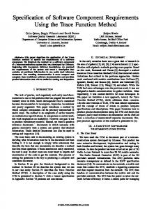
¡ ¢ ¡ ¢ where k2 denote the binomial coefficient k2 = k(k−1) . 2 ¡k¢ The value 2 corresponds to the maximum number of edges that can connect vertices in N (v) (the number of edges in the complete graph on the set of vertices Nv ). So the metric measure the edge density in the neighborhood of the vertex v. Figure 2 illustrates the calculation of this metric. The value c(v) represents the ratio of the actual number

lirmm-00269464, version 1 - 3 Apr 2008

Av. path length 3.28 3.96 3.78 3.60 2.86 3.02 2.46 2.8

Table 1. Cluster measure and average path length of several software systems.

1_ 2

v

Cluster measure 0.95 0.15 0.108 0.129 0.387 0.099 0.725 0.016

| Nv | = 5

1_ 2

1 _ 2

e 1_ 2

e(Nv) = 4

1_ 2

1_ 2

1_ 2

G

1 _ 2

Figure 3. Isthmus.

Figure 2. Calculation of the clustering metric.

of edges between vertices of Nv in relation to the maximal number of edges between these vertices. Since there are 4 edges connecting neighbors of v (darker edges), we have 4 c(v) = 10 .The clustering measure of a graph G is obtained by averaging the clustering measure of all vertices,

2.2 Edge strength metric We now extend the metric c to a metric Σ defined on edges of a graph. As we will see, this new metric has many interesting properties for metric based clustering of graphs. In particular, it resolves the situation we pointed at above since it is such that Σ(e) = 0 if e is an isthmus. This metric corresponds to a measure of how much an edge is likely to separate a graph in two highly connected subgraphs. It measures the strength of edges in regard to this property. This metric is related to the density of edges in the neighborhoods of the end vertices of e, and thus appears as a generalization of the cluster measure to edges in a graph. As we will see, this density is calculated from the ratio of the number of paths of length three and four actually going through e in relation to the maximal number of such paths. We need to introduce notations before we can describe our extension of c to edges. Let e be an edge and u, v be its endpoints. Denote by Nu and Nv the respective neighborhoods of u and v and define the set Mu = Nu \ Nv . The set Mu contains neighbors of u that are not neighbors of v. Similarly, define Mv = Nv \ Nu . Moreover, let Wuv be the intersection of Nu and Nv . That is, Wuv gathers vertices that are neighbours of both u and v. Observe that the sets Nu , Nv and Wuv form a partition of the set of vertices at distance 1 from u or v. Figure 4 summarizes the situation. This partition is useful to classify cycles of length four (4cycles) going through the edge e. First observe that such a cycle contains four vertices. Two of them are u and v, so

1 X c(v). |G| v∈G

Small-world graphs are graphs with high cluster measure and small average path length, in comparison to the same statistics computed on random graphs (see [8] and [9]). That is, these graphs correspond to networks where any two nodes are only a few steps away from each other, and where nodes are globally organized as closely linked subgroups. Table 2.1 reports those measures for several software systems, as well as for random graphs, providing arguments to the fact that software systems define small-world graphs. The idea we started from was to exploit the cluster measure of vertices to detect clusters in a graph. However, the cluster measure on vertices does not reveal itself as a good indicator. Indeed, Figure 3 shows a graph where several different vertices are assigned the same cluster measure. Thus, the metric indicates that all vertices with a metric value of 1/2 play similar or equivalent roles in the graph. However, one can argue that the left and right groups of vertices are its natural clusters and that the central edge weakly links them. Hence, we seek for an edge measure that would identify the central edge e as the one to be removed. 3

corresponding to 4-cycles going through an edge e = u, v

Wuv

Mu

γ4 (e) = s(Nu , Wuv ) + s(Nv , Wuv ) + s(Nu , Nv ) + s(Wuv ).

e u

v

Similarly, edge density related to 3-cycles going through e can be computed as

...

...

...

Mv

γ3 (e) =

|Wuv | . |Wuv | + |Nv | + |Nv |

Finally, the strength metric of an edge e is defined as the sum:

Figure 4. Partition used to calculate the strength metric of an edge.

lirmm-00269464, version 1 - 3 Apr 2008

Σ(e) = γ3 (e) + γ4 (e) the two remaining vertices x and y are necessarily included in the sets Nu , Nv or Wuv . Hence, we can classify 4-cycle depending on which of these sets the two other vertices belong. There are four possibilities.

This definition is related to edge density in the neighborhood of e (where the neighborhood has been divided into three distinct parts as above). A low value for Σ(e) indicates that the edge is more likely to act as an isthmus between clusters. Contrarily, a high value for Σ(e) indicates that it is potentially at the center of a cluster. Consequently its endpoints and possibly its neighborhood should belong to a same cluster. It is worth to note that the metric Σ is related to the notion of shortcut used in the context in small-word graphs (see [8]). In fact, the value of Σ(e) will be high if the edge e is a shortcut for many 3-cycles and 4-cycles passing through e. The value will be low if there is not so many cycles of length 3 and 4 passing through e.

Wuv

e Mu

u

v

Mv

Figure 5. A 4-cycle through e. Figure 5 illustrates one of them, namely the situation where the 4-cycle is completely determined by an edge x, y connecting a vertex from Wu,v to one in Mv . The three other possibilities correspond to situations where x ∈ Mu and y ∈ Wu,v , or x ∈ Mu and y ∈ Mv , or x, y ∈ Wuv . Let U and V be two subset of vertices. Define the ratio s(U, V ) =

Figure 6. Extraction of clusters.

e(U, V ) . |U | |V |

Figure 6 result from the application of the metric Σ to the edges of a graph. The thickness and saturation of an edge reflect the value of the metric. Edges with higher values are wider and darker blue, while edges with low values are thinner and lighter. From the figure, it is clear that the deletion of thinner and lighter colored edges separates the graph into two clusters. The graph was laid out using a forcedirected algorithm, naturally grouping vertices of a same cluster close together, confirming the predicted ability of the metric. Computational complexity issues concerning the metric Σ are addressed in an appendix at the end of the paper.

where e(U, V ) denotes the number of edges connecting a vertex of U to a vertex in V . Thus s(U, V ) computes the ratio of the actual number of edges between the sets U and V with respect to the maximum number of possible edges between those two sets. Also, we define e(U ) s(U ) = ¡|U |¢ . 2

Using our notations, we can express the edge density γ4 (e) 4

3 Applications

3.2 Calculation on graphs related to physical design

In this section, we present applications of our clustering technique to existing software systems, showing the relevancy of our method to reverse software engineering. In all examples shown, graphs have been laid using a forcedirected algorithm. Moreover, the thickness and saturation of an edge e have been assigned according to its metric value Σ(e).

We have applied our method to the graph resulting from the include relations between source files of the MacOS9 operating system API. This API called Universal Headers is publicly available at the URL http://developer.apple.com/sdk. Includes relations are induced by the #include pre-compiler directive in C++. Figure 8 illustrate the clusters calculated with our technique. The threshold value used here has been chosen as described in Section 4.2. In Figure 8, every file in the cluster labelled

lirmm-00269464, version 1 - 3 Apr 2008

3.1 Calculation on graphs related to logical design: Access graphs Our first example shows the application of the metric Σ to the edges of the access graph of the ResynAssistant software, written in Java at LIRMM. This software is dedicated to organic chemistry. Vertices of this access graph are Java classes. There is an edge between two classes if one of them has access to a method of the other. The access graph presented here have been generated from the work of by Ardourel et al. [10] The graph is shown in Figure 7.

Figure 8. Clusters in MacOS9. CG belong to the Core Graphics component of MacOS. The cluster labelled CF contains files belonging to the Core Foundation Utility Routines component. Another cluster is labelled QT and corresponds to QuickTime. Many of the files in the cluster labelled ATS are related to the Apple Type Services component. Note however that there are files not directly in this component (for example, a file belonging to this cluster is related to threads). Remark that software components are less easily extracted from the include relations on source files, since this relation actually reflects the way the software is implemented. The next example is about Microsoft Foundation Classes (MFC). We have applied our algorithm to the graph resulting from the include relations between source files. Figure 9 illustrate the result. The larger cluster, labelled AFX,ATL contains file from the Application Framework and Active Template Library components of MFC. Another cluster, labelled OCC, contains files from OLE Container Component. A small cluster concerns the strings mapping component. It is labelled MAP. Finally, we have found a cluster related to data base support, labelled DBSup, which contains

Figure 7. Application of the metric to ResynAssistant software.

In this example, clusters extracted with our technique have been placed in boxes. The name of the respective packages is indicated in Figure 7. The designers have confirmed that the clusters we were able to identify correspond to the logical structure of the source code. Incidentally, the visualization of the access graph and a close study of the clustering led them to the identification of a design error. More precisely, the cluster labelled Others classes appear as a single cluster instead of two because of loosely designed accesses. 5

a few files. The two previous clusterings contain many iso-

two partitions. For instance, there is no immediate conclusion to draw from a negative M Q value, or from a low positive value. This would be possible only if we could assert that there are many other possible partitions with a much higher value. We have addressed this problem by looking at the range of all possible M Q values, for a wide subset of partitions of a graph G chosen randomly from the set of all possible partitions. The M Q values were then collected into a histogram showing their frequencies among the chosen subset of partitions. It turns out that this histogram can be approximated using a gaussian distribution (see Figure 10).

2

1.5

lirmm-00269464, version 1 - 3 Apr 2008

Figure 9. Clusters in MFC.

1

lated vertices. This is related to the structure of the system which can be seen as a collection of overlapping subtrees. The threshold value used in the calculation of the previous clusters was obtained by the method described in section 4.2.

0.5

–1

M Q(C; G) =

s(Ci , Ci ) − p

Pp−1 Pp i=1

–0.4

-0.2

0

0.2

0.4

0.6

0.8

1

Figure 10. MQ distribution.

We now turn ourselves to the problem of evaluating the quality of a clustering of a graph. This problem has been previously addressed by a number of people in the software engineering community [5, 2, 3]. From all the quality measures that have been defined, we focus on M Q introduced by the authors of [3]. M Q actually computes a value for any given partition C = (C1 , . . . , Ck ) of a graph G = (V, E). Edges in E contribute as a positive or negative weight according to whether they are incident to vertices of a same block Ci or to vertices of distinct blocks Ci , Cj . It is defined as follows, using the notations introduced in section 2.

i=1

–0.6

x

4 Clustering quality measures

Pp

–0.8

j=i+1

s(Ci , Cj )

p(p − 1)/2

The proof of this fact is somewhat straightforward and is a consequence of the central-limit theorem [11]. Indeed, each of the terms s(Ci , Ci ) in Equation 1 can be seen as a random variable. These random variables are obviously independent (since they concern disjoint sets of edges) and have a mean and standard deviation that converge to the same values (as the number of vertices in the graph grows larger). So the central-limit theorem applies and we get that the left ratio in Equation 1 indeed converges towards a gaussian distribution. The same argument applies to show that the second ratio on the right also converges to a gaussian distribution. Finally, these two gaussian variables are independent, so their sum is also a gaussian distribution. (See [11] for more details.) Moreover, the mean value and standard deviation of this gaussian approximation can be satisfactorily estimated as µ = −0.2 and σ = 0.2 as indicated in Figure 10. This result can now be used to answer the questions we pointed at above. Given a partition C, we are now able to judge of its goodness or badness with more confidence. For instance, choosing a partition uniformly at random will most surely give a clustering with a negative M Q value close to −0.2. Conversely, a partition with a positive but even small value, is already a good clustering of a graph (compared to what an average partition would give). Indeed, the probability that a

.

(1) A straightforward consequence is that a higher M Q value can be interpreted as better since it corresponds to a partition with either fewer edges connecting vertices from distinct blocks, or with more edges lying within identical blocks of the partitions, which is what most clustering algorithms aim at finding. A straightforward consequence of this definition is that M Q always lies in the [−1, 1] interval. However, this feature of M Q being normalized to the [−1, 1] interval does not provide enough information to assess of the good or bad quality of a partition, and compare 6

lirmm-00269464, version 1 - 3 Apr 2008

random partition has a positive value is approximately 15%. A bit more than 10% of all partitions have an M Q value above 0.05 and only 2% of all partitions have an M Q value above 0.2. A partition with an M Q value above 0.31 can only be found in 0.5% of all partitions. Remark The above definition for M Q actually differs from the one used in [6]. Contrarily to Bunch, we chose to define M Q for undirected graphs. This choice does not affect the definition of the numerators but only changes the denominators (which differ by a factor 1/2). This makes sense since some of the graphs we study correspond to the non-symmetric “includes” relations between physical files. The graph for the ResynAssistant API is obtained differently. The vertices of the graph correspond to classes of the API. A vertex u is adjacent to a vertex v if it can access methods or attributes of v. Although the edges of the graph have natural orientations, we ignored them and considered the graph as non-directed.

clusterings. Graph ResynAssistant (access) Mac OS9 (includes) MFC (includes) Random clustered

MQ/Bunch 0.435 (10) 0.137 (4) 0.044 (4) 0.322 (6)

MQ/Strength 0.368 (10) 0.015 (251) 0.011 (373) 0.346 (6)

Table 2. Comparison of M Q values between Bunch and Strength metric Table 4.1 shows that, in most cases, the clustering obtained from the Strength metric compares well with the one obtained from Bunch, since both clusterings have very close M Q values. For instance, the results obtained for the ResynAssistant API compare very well, since the subset of partitions having an M Q value lying between 0.368 and 0.435 represents only a bit more that one tenth of a percent of all partitions. it should also be remarked that in both cases the partitions found consist of the same number of blocks. The bad comparison for the Mac OS9 and MFC softwares admits a simple explanation. The structure of these graphs roughly compares with a large and highly coupled component having several and smaller hierarchies attached to its periphery. To be able to get at the 4 components identified by Bunch, our method needs to filter the edges with a high threshold value, thus leaving a rather large number of nodes isolated. Each of these nodes corresponds to a cluster, and edges stemming from them count as inter-cluster, which explains the bad M Q score we get. Collecting the isolated nodes and grouping them to one of the four larger components (through a DFS for instance) would undoubtedly lead to a better M Q value and to a much lower number of clusters. The random clustered graph example (see Figure 1) was run for sake of completeness. This graph, although not random from a strictly theoretical point of view, is built by selecting a number of clusters, prescribing upper and lower bounds for their number of inter-cluster edges and extracluster edges. It is not at all surprising that both methods find a clustering with the exact number of blocks. The surprise is that with this example, our method was able to obtain a better score than Bunch. In another random clustered example, not reported here, both methods found exactly the same clustering.

4.1 Links between M Q and the strength metric for edges We now look at the quality of the clustering obtained by filtering the graph with the strength metric. The question we examine here is ‘Just how good is the clustering obtained by filtering out the edges ?’ As a first evaluation, we have compared the clusterings we obtain with the ones produced by Bunch [6], which appears as one of the good clustering software used by the reverse engineering community. It should be well understood that our method does not compete with Bunch. As we understand it, Bunch implements standard optimization methods and tries to find a clustering with the highest possible M Q value. The value of our approach, as we shall see, is that it produces clustering of good quality in short computing time, since it has low computational complexity. In our view, our technique could be used to significantly improve the performance of Bunch or similar tools or algorithms. Indeed, starting the search for a good clustering with an already good candidate usually improves the performance of such algorithms, both in time and quality. Moreover, our technique can be embedded in an interactive environment to let the user guide Bunch (or any other software based on heuristic algorithms) find a good clustering candidate in the minimum time. The following table summarizes the comparisons we made with Bunch. The quality measures we report should be interpreted in view of the statistical distribution of the M Q values we underlined in the preceding section. For each software system we examined, we report the M Q value of a clustering found by Bunch and the clustering induced from the strength metric (using the best possible threshold value). The figures in parenthesis report the number of blocks in the

4.2 Automating the process We have mentioned that our method could well be embedded in an interactive environment, giving a user the freedom to browse through the clusterings we are able to produce. However, when considering our method as a possible input for Bunch, we need to be able to automatically identify the 7

lirmm-00269464, version 1 - 3 Apr 2008

clustering to use as a starting point. This problem translates into the question of finding the threshold value corresponding to the clustering with the highest possible M Q score we are able to find. Hence we were naturally led to study the possible correlation between the interval of thresholds and the M Q values we reach. Figure 11 shows the variation of M Q as the threshold goes through the interval of all possible values for the strength metric. The metric values on the x-axis have been normalized to the [0, 1] interval. The curve gives the M Q score associated with the clustering obtained from the corresponding threshold value on this interval. The variation along the curve also relates to a path in the set of all possible partitions. Indeed, suppose a threshold value t ∈ [0, 1] has been chosen and denote by Ct the clustering induced from this threshold t. Then, the clustering Ct0 induced from a slightly larger threshold t0 > t can be obtained from Ct by dividing some of its blocks into two or more parts. Hence the ordered list of all clusterings obtained by letting t vary over the whole interval [0, 1] gives an ascending path in the lattice of all partitions. That is, the path corresponds to a curve extracted from a high-dimensional space (the space of all possible partitions and their corresponding M Q value).

of times).

Mac OS9 (includes)

0.025

0.02

MQ

0.015

0.01

0.005

0

0.2

0.4

0.6

0.8

Strength –0.005

Figure 12. MQ/Strength plot for Mac OS9 includes.

It should be remarked at this point that the MQ values reported in the comparison table in section 4 have been computed by Bunch. However, the curves in Figure 11 and Figure 12 report values computed with our version of M Q, (which basically explains why the maximum M Q values reached by the curves is relatively higher).

ResynAssistant API

0.8

0.6 MFC (includes)

MQ 0.4 0.05

0.2 0.04

0

0.2

0.4

0.6

0.8

Strength

MQ

0.03

–0.2 0.02

0.01

Figure 11. MQ/Strength plot for the ResynAssistant API.

0

0.2

0.4

0.6

0.8

Strength

Figure 13. MQ/Strength plot for MFC includes.

As Figure 11 shows, once the curve has been computed, it is straightforward to find its maximum value. It could actually be useful to find all local maxima which can be indicators for good clustering candidates (a local maxima could just be a point sitting close to a peak reached by the curve). Indeed, the MQ/Strength curve can admit many local maxima, as shows Figure 12. Also, it should be noted that the cost for computing the curve is proportional to the cost of computing M Q for a given partition of a graph (since the [0, 1] interval is interpolated at values t a constant number

Figure 13 shown as last example the graph of includes for the MFC API (see Figure 9). Again, the local maxima can be easily computed in order to get at a almost optimal clustering of the graph. Note however that the intrinsic structure of the graph makes it difficult to reach high M Q scores. We also ran this example with Bunch who produced clusterings having an M Q value just above zero, even by letting the 8

heuristics run extensively. In situations such as this, our method seems to offer a tangible advantage, be it simply that it can find similar candidates almost instantly.

Working Conference on Reverse Engineering, October 1999. [3] B. S. Mitchell and S. Mancoridis, “Comparing the decompositions produced by software clustering algorithms using similarity measurements,” in ICSM, pp. 744–753, 2001.

lirmm-00269464, version 1 - 3 Apr 2008

5 Perspectives and future work We have presented a simple, fast computing and easy to implement method aiming at the capture of software components from a logical and physical point of view. Our method exploits a metric based clustering of graphs. The metric we have introduced is a new metric that measures edge density in graphs and is inspired from the cluster measure defined by Watts [9] for the so-called small-world graphs. The motivation behind this is that software systems show resemblance with graphs of this class. The relatively low complexity of the underlying calculations of our method allows it to be embedded in an interactive environment. Clusters on graphs of thousands of vertices can be done in a second. From the experimentations we were able to conduct, our method appears to get better results for graphs corresponding to logical design that those resulting from physical design. Indeed, the graphs resulting from include relations do not always separate into well defined and large clusters but tend to explode into several small clusters. This is a consequence of the fact that the graph under study often depends on the quality of the underlying software. It should be mentioned that although our method does not appear as being well adapted to repair deficient design, it is useful to detect design flaws. We have mentioned that our method appears as a useful preprocess step to optimization procedures such as the ones used by Bunch. More work is needed to demonstrate the use of our technique as a guiding strategy or as good initial solutions for optimization heuristics. This study should most probably go deeper into the comprehension of the structure of the space of all clusterings, with respect to M Q seen as a similarity measure. Also, the actual quality of the clusterings we are able to produce suffer from the large number of isolated vertices. The quality can certainly be improved by agglomerating them to larger clusters using a DFS for instance.

[4] C. F. N. Anquetil and T. C. Lethbridge, “Experiments with hierarchical clustering algorithms as software remodularization methods,” in WCRE’99, 1999. [5] R. Koschke and T. Eisenbarth, “A framework for experimental evaluation of clustering techniques,” in International Workshop on Program Comprehension (I. C. S. Press, ed.), pp. 201–210, 2000. [6] S. Mancoridis, B. Mitchell, Y. Chen, and E. R. Gansner, “Bunch: A clustering tool for the recovery and maintenance of software system structures,” pp. 50–62, IEEE Proceedings of the 1999 International Conference on Software Maintenance (ICSM’99), August 1999. [7] B. Mirkin, Mathematical Classification and Clustering. Kluwer Academic Publishers, 1996. A textbook with many practical examples. [8] D. J. Watts and S. H. Strogatz, “Collective dynamics of small-world networks.,” Nature, vol. 393, pp. 440– 442, 1998. [9] D. J. Watts, Small World. Princeton University Press, 1999. [10] O. Gout, G. Ardourel, and M. Huchard, “Access graph visualization: A step towards better understanding of static access control,” in Electronic Notes in Theoretical Computer Science (T. M. Gabriele Taentzer and A. Sch¨urr, eds.), Elsevier Science Publishers, 2002. [11] W. Feller, An Introduction to Probability Theory and Its Applications, vol. 1. Wiley Science, 1968.

References [1] S. Mancoridis, B. Mitchell, C. Rorres, Y. Chen, and R. Gansner, “Using automatic clustering to produce high-level system organizations of source code,” pp. 45–53, IEEE Proceedings of the 6th Int. Workshop on Program Understanding, June 1998. [2] V. Tzerpos and R. Holt, “Mojo : A distance metric for software clustering,” pp. 187–193, Proceedings of the 9

6 Appendix: Complexity analysis 6.1 Strength measure Let G = (V, E) be a graph and write |V | = n and |E| = m. Also, assume thatP the average degree of vertices is bounded

lirmm-00269464, version 1 - 3 Apr 2008

d(v)

≤ c, where c > 0 is a positive by above, that is v∈V n real number. Note that this assumption follows from empirical observations applies to all software systems that we studied. Let e ∈ E be an edge in the graph. The computation of the metric boils down to the computation of the seven sets Mu , Mv , Wuv (described in section 2.2), E(Mu , Mv ), E(Mu , Wuv ), E(Mv , Wuv ) and E(Wuv ). The computation of the first three sets is made in constant time, by virtue of the assumption on the average degree of vertices. The four last sets are built by looking at the neighborhood of all vertices belonging to Mu , Mv and Wuv . Note that, the average size of each of these three sets is at most c. Hence, the computation of each of the set E(U, V ) (where U, V stand for the appropriate neighborhoods) is done in time at most c2 on average. To sum up, building the seven sets is made in constant time O(c2 + c). Consequently, the metric is computed on the whole graph in time O(m) (observe that our assumption on the average vertex degree implies that m is proportional to n).

6.2 Cluster retrieval We now look at the actual cost for computing the clusters induced from a fixed threshold value t ∈ [a, b]. Note that this can be done through a Depth First Search algorithm. The complexity of this algorithm is O(N + M ).

10