Software Development Effort Estimation using Fuzzy ...

Software Development Effort Estimation

Chakraborty and Patnaik

Software Development Effort Estimation using Fuzzy Bayesian Belief Network with COCOMO II B.Chakraborty

(1),

K.S.Patnaik

(2)

(1) Department of Computer Science and Engineering.Birla Institute of Technology, Mesra (India) E-mail: [email protected] (2) Department of Computer Science and Engineering. Birla Institute of Technology, Mesra (India) E-mail: [email protected]

ABSTRACT Software development has always been characterized by some metrics. One of the greatest challenges for software developers lies in predicting the development effort for a software system which is based on developer abilities, size, complexity and other metrics. Several algorithmic cost estimation models such as Boehm’s COCOMO, Albrecht's' Function Point Analysis, Putnam’s SLIM, ESTIMACS etc. are available but every model has its own pros and cons in estimating development cost and effort. Most common reason being project data which is available in the initial stages of project is often incomplete, inconsistent, uncertain and unclear. In this paper, Bayesian probabilistic model has been explored to overcome the problems of uncertainty and imprecision resulting in improved process of software development effort estimation. This paper considers a software estimation approach using six key cost drivers in COCOMO II model. The selected cost drivers are the inputs to systems. The concept of Fuzzy Bayesian Belief Network (FBBN) has been introduced to improve the accuracy of the estimation. Results shows that the value of MMRE (Mean of Magnitude of Relative Error) and PRED obtained by means of FBBN is much better as compared to the MMRE and PRED of Fuzzy COCOMO II models. The validation of results was carried out on NASA-93 dem COCOMO II dataset. Keywords: Bayesian Belief Network, COCOMO II, Fuzzy Set, Software Development Effort, Agena Risk

1- INTRODUCTION Estimating the Effort of a Software development project remains a challenge for the researchers. Despite the various methods proposed, unsolved questions and problems justify further research and experimentation. The diversity of cost factors, their unclear contribution to effort and the lack of information in the early stages of software development are the main components of the problem, classifying it to probabilistic reasoning. The most critical issue in this

3

Int. J. of Software Engineering, IJSE Vol.8 No.1 January 2015

scientific endeavour is the agreement on the constituent, pertinent elements of the problem. Classical methods demand simple linear structures and a wealth of data often missing in software engineering. A flexible and competitive method to the above methods is Bayesian Belief Networks (BBN) [1]. Graphical models such as BBN have become attractive tools because of their ability to efficiently perform reasoning tasks and to represent uncertainty in expert systems. There are several software effort estimation techniques reported in the literature. Among a few popular techniques are linear regression models, cost models (COCOMO/COCOMO II, SLIM, etc.) [2][3][4], neural network models, and vector prediction models. Accuracy in software estimation is among the greatest challenges for software developers. Software effort estimation deals with the prediction of the probable amount of time and cost required to complete the specific development task. Software metric and especially software estimation is based on measuring of software attributes which are typically related to the product, the process and the resources of software development. This paper extends the Constructive Cost Model (COCOMO II) by incorporating the concept of fuzziness and uncertainity in terms of Bayesian Belief Networks. Here, the key cost drivers are identified [5] and Fuzzy Bayesian approach was used to obtain their accurate values. The paper is organized as follows: section II briefly outlines the cost estimation models and COCOMO II model. Section III discusses implementation of FBBN methodology in COCOMO II model. Section IV concludes with evaluation of numerical simulation result and its comparison with existing methods.

2- SOFTWARE EFFORT ESTIMATION MODELS Software developers’ estimates time of software tasks by comparing similar tasks that have already been developed. Its purpose is to accurately estimate the resources needed and required schedules for software development projects. The software estimation process includes estimating the size of the software product to be produced, estimating the effort required, developing preliminary project schedules, and finally, estimating overall cost of the project [6]. Although, this task has an uncertain nature, due to its dependency on several and usually not clear factors and which is hard to be modeled mathematically [7]. For considerable financial and strategic planning, the reliable and accurate cost estimation is an ongoing challenge. Software effort estimation models are divided into two main categories: algorithmic models and nonalgorithmic models.

2-1 ALGORITHMIC MODELS Algorithmic models are designed in such a way that they provide a mathematical equation which is based upon the statistical analysis of data gathered from previously developed projects, e.g. Software Life Cycle Management

4



(SLIM) [2] and COCOMO [3][4] and Albrecht’s Function Point. These mathematical equations use inputs such as Source Lines of Code (SLOC), number of functions to perform / number of user screen, interfaces, complexity, and other cost drivers such as language, design methodology, skill-levels, risk assessments, etc. at a time when uncertainty is mostly present in the software [8][9]. As most of the software development effort estimates are based on the prediction of size of the system to be developed but this is a difficult task as the estimates obtained at the early stages of development are more likely to be inaccurate because not much information of the project to be developed is available at that time. So the correctness of model largely depends upon the information that is available during the preliminary stages of development. Now considering the current technological advancements these algorithmic models are unable to provide a suitable solution. Though these models may be good enough to handle a particular environment but they are not flexible enough to adapt new environment. The inability of algorithmic model to handle categorical data (which are specified by a range of values) and most importantly lack of reasoning capabilities contributed to the number of studies exploring non-algorithmic methods [10].

2-2 NON-ALGORITHMIC MODELS Non-algorithmic models came in 1990’s and widely used in software cost estimation. Software researchers looked for new approaches which were based on soft computing approach such as artificial neural networks, Fuzzy logic, and genetic algorithms. Fuzzy Logic offers a powerful linguistic representation that able to represent imprecision in the model inputs and outputs, while providing a more knowledge base approach to establish an effective model. Research shows that using Fuzzy Logic can result in good performance in terms of reducing imprecision of inputs and outputs parameters.

2-2-1 COCOMO II The COCOMO I model is a regression-based stable software cost estimation model developed by Boehm in 1981. One of the problems with the use of COCOMO I today is that it does not match the development environment of the late 1990’s. Therefore, in 1997, Boehm developed the COCOMO II which solved most of the COCOMO I problems. The estimated effort is given by equation 1 and equation 2 refers to the scaling exponent used in COCOMO II. The COCOMO II includes several software attributes such as: 17 Effort Multipliers (EMs), 5 Scale Factors (SFs), Software Size (SS), and Effort estimation that are used in the Post Architecture Model of the COCOMO II. The description of the 17 EMs and 5 SFs based upon their numerical values and productivity ranges are shown in Table 1 and Table 2.

5


Table 1 - The Range of COCOMO II EMs

Effort Multiplier

Range

Required s/w reliability (RELY) Database size (DATA) Product complexity (CPLX) Developed for reusability (RUSE) Documentation match to life-cycle need (DOCU) Execution time constraint (TIME) Main Storage constraint (STOR) Platform volatility (PVOL) Analyst capability (ACAP) Programmer Capability (PCAP) Personnel Continuity (PCON) Application experience (APEX) Platform experience (PEXP) Language and tool experience (LTEX) Use of software tools (TOOL) Multi site development (SITE) Required development schedule (SCED) ‘

0.75 - 1.39 0.93 - 1.19 0.75 - 1.66 0.91 - 1.49 0.89 - 1.13 1.00 - 1.67 1.00 - 1.57 0.87 - 1.30 1.50 - 0.67 1.37 - 0.74 1.24 - 0.84 1.22 - 0.81 1.25 - 0.81 1.22 - 0.84 1.24 - 0.72 1.25 - 0.78 1.29 - 1.00

Table 2 - The Range of COCOMO II SFs

Scale Factors

Range

Precedentness(PRED) Development Flexibility(FLEX) Architecture/Risk resolution(RESL) Team cohesion(TEAM) Process maturity(PMAT)

6.20 - 1.24 5.07 - 1.01 7.07 - 1.41 5.48 - 1.10 7.80 - 1.56

Above scale factors ranges from very low to very high. Extra high value of the scale factors is 0.

3- PROPOSED APPROACH 3-1 BAYESIAN BELIEF NETWORK Bayesian Belief Network (BBN) [1][9][11][12][13][14][15] is a directed Acyclic Graph with nodes representing variables, and arcs represent conditional dependence. Software development project is a collection of efforts and resources in a defined time period to realize a software product which satisfies the requirements made by a client or agreed upon [8][11]. Project management focuses on suitable application of efforts and resources to achieve the constraints of Cost, Time and Quality. From very first day, the planning for ef-

6



forts and resources is conducted based on estimates. Estimation is the key to planning and is made not only at the beginning but also at every single milestone. Current research in estimation is focused on issues like development of new models, metrics conversion, uncertainty, missing data, intelligent decision support and models for new life cycles [8][11][12][13][14]. In software development effort estimation, a large set of factors has been identified [8][9] which affects the final effort and the productivity of the organization. This set of factors reaches up-to 20 in some studies [9]. However incase of BBN development we need to keep one critical issue i.e. size of model. The size of Bayesian Belief network model increases the computational requirements [15], so, we need to select a minimal set of factors which represent the problem.

3-2 FUZZY BAYESIAN BELIEF NETWORK (FBBN) MODEL USING COCOMO II According to Bohem, each Post-Architecture cost driver in COCOMO II model is measured using a rating scale of 6 linguistic values, such as “Very Low”, “Low”, “Nominal”, “High”, “Very High, and “Extra High. The corresponding linguistic values use the conventional quantification approach when it is assigned, and it is represented by crisp intervals.

In our model the range of EMs are taken as distribution of their possible values instead of constant values. This reduces the traditional problem of software effort estimation dependency on single value.

According to [5], all the effort multipliers are not equally important, hence only 6 key cost drivers among 17 cost drivers is considered here.The six key cost drivers are categorized under 2 factor: RELY (Required s/w reliability), CPLX (Product complexity) and TIME (Execution time constraint) together form Product Factor; ACAP (Analyst Capability), PCAP (Programmer Capability) and PCON (Personnel Continuity) together form Personnel Factor [5].These six cost drivers were found more significant using Monte Carlo Simulation technique[5]. 3-2-1 Fuzzification Fuzzy logic helps in situations where the uncertainty exists in the form of possibility. Fuzzy logic provides different fuzzy functions which can be used to map the uncertainty [16]. We use the symmetrical triangular membership function of fuzzy logic which provides a triangular possibility distribution. (3)

7


Where, ‘m’ is the central value, ‘a’ is the lower limit and ‘b’ is the upper limit.

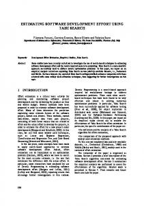
Figure 1 - FBBN COCOMO II Model

Figure 1 depicts the framework used for estimation.The TIME, RELY and CPLX are the inputs to the first DAG named Product along with a fuzzy node so as to get value of the product factor and PCAP, PCON and ACAP are inputs to second DAG named Personnel along with a fuzzy node so as to get value of the personnel factor. The framework deals with fuzzy bayesian modeling of the key cost drivers. The size and scale factors are inputs to the third DAG named SF(1-3) and fourth DAG named E1. The Product factor and Personnel Factor and the output of the fourth DAG are inputs to the fifth and final DAG named effort whose output gives us the value of the software development effort.

Figure 2 - DAG showing the FBBN for Product Factor

8



Table 3 - Nodes for DAG representing Product Factor

Sl. No. 1 2

Node CPLX CPLX_2

3 4

RELY RELY_2

5 6

TIME TIME_2

7 8

FUZZY PRODUCT_FACTOR

Type Manual Partitioned Expression Manual Partitioned Expression Manual Partitioned Expression Manual Expression

NPT Table 8 Table 9 Table 10 Table 11 Table 12 Table 13 Table 14 Triangle((1)*cplx*rely1*time, (1+ )*cplx*rely1*time, cplx*rely1*time)

Figure 3 - DAG showing the FBBN for Personnel Factor Table 4 - Nodes for DAG representing Personnel Factor

Sl. No. 1 2

Node ACAP ACAP_2

3 4

PCAP PCAP_2

5 6

PCON PCON_2

7 8

FUZZY PERSONNEL_FACTOR

Type Manual Partitioned Expression Manual Partitioned Expression Manual Partitioned Expression Manual Expression

NPT Table 10 Table 15 Table 10 Table 16 Table 10 Table 17 Table 14 Triangle((1)*acap*pcap*pcon, (1+ )*acap*pcap*pcon, acap*pcap*pcon)

9


Figure 4 - Depicting the DAG for the first three SFs Table 5 - Nodes for DAG representing 3 Scale Factors

Sl. No. 1 2

Node PREC PREC_2

3 4

FLEX FLEX_2

5 6

RESL RESL_2

7

SCALE1

Type Manual Partitioned Expression Manual Partitioned Expression Manual Partitioned Expression Expression

NPT Table 8 Table 18 Table 8 Table 19 Table 8 Table 20 Arithmetic(prec+flex+resl)

Figure 5 - Depicting the DAG rest of the SFs and the size

10



Table 6 - Nodes for DAG representing rest of the Scale Factors and size

Sl. no. 1 2 3 4 5 6 7

Node PMAT PMAT_2 TEAM TEAM_2 SCALE1 SCZ(SIZE) SCALE2

Type Manual Partitioned Expression Manual Partitioned Expression Expression Expression Expression

NPT Table 8 Table 21 Table 8 Table 22 Uniform(0,20) Uniform(1,1000000) Arithmetic(2.94* (size^(0.01*(team+pmat+S CALE1)+0.91)))

Figure 6 - DAG representing the final effort Table 7 - Nodes for DAG representing final effort

Sl. No. 1

Node SCALE2

Type Expression

2 3 4

PERSONNEL_FACTOR PRODUCT_FACTOR EFFORT

Expression Expression Expression

NPT Uniform(0,1000000) Uniform (0,8) Uniform (0,8) Arithmetic(SCALE2* PER_FAC*PRO_FAC)

Table 8 - NPT showing the node states from VL to EH and their respective probabilities

Node States Very Low(VL) Low(L) Nominal(N) High(H) Very High(VH) Extra High(EH)

Probability 0.16666667 0.16666667 0.16666667 0.16666667 0.16666667 0.16666667

11


Table 9 - NPT for CPLX_2

Node States Very Low(VL) Low(L) Nominal(N) High(H) Very High(VH) Extra High(EH)

Expression Triangle(0.7,0.8,0.73) Triangle(0.8,1,0.87) Arithmetic(1) Triangle(1.15,1.3,1.2) Triangle(1.3,1.43,1.34) Triangle(1.5,2,1.74)

Table 10 - NPT showing the node states from VL to VH and their respective probabilities

Node States Very Low(VL) Low(L) Nominal(N) High(H) Very High(VH)

Probability 0.2 0.2 0.2 0.2 0.2

Table 11 - NPT for RELY_2


Expression Triangle(0.8,0.9,0.82) Triangle(0.9,1,0.92) Arithmetic(1) Triangle(1.1,1.25,1.2) Triangle(1.25,1.5,1.26)

Table 12 - NPT showing the node states from N to EH and their respective probabilities

Node States Nominal(N) High(H) Very High(VH) Extra High(EH)

Probability 0.25 0.25 0.25 0.25

Table 13 - NPT for TIME_2

Node States Nominal(N) High(H) Very High(VH) Extra High(EH)

12

Expression 0.25 0.25 0.25 0.25



Table 14 - NPT for FUZZY

Node States 0-0.2 0.2-0.4 0.4-0.6 0.6-0.8 0.8-1.0

Probability 0.2 0.2 0.2 0.2 0.2

Table 15 - NPT for ACAP_2



Table 16 - NPT for PCAP_2



Table 17 - NPT for PCON_2

Node States Very High(VH) High(H) Nominal(N) Low(L) Very Low(VL)


Table 18 - NPT for PREC_2

Node States Extra High(EH) Very High(VH) High(H) Nominal(N) Low(L) Very Low(VL)

Expression Arithmetic(0) Arithmetic(1.24) Arithmetic(2.46) Arithmetic(3.72) Arithmetic(4.96) Arithmetic(6.2)

13


Table 19 - NPT for FLEX_2



Table 20 - NPT for RESL_2



Table 21 - NPT for TEAM_2

Node States

Expression

Extra High(EH) Very High(VH) High(H) Nominal(N) Low(L) Very Low(VL)

Arithmetic(0) Arithmetic(1.1) Arithmetic(2.19) Arithmetic(3.29) Arithmetic(4.38) Arithmetic(5.48)

Table 22 - NPT for PMAT_2

Node States

Expression

Extra High(EH) Very High(VH) High(H) Nominal(N) Low(L) Very Low(VL)

Arithmetic(0) Arithmetic(1.56) Arithmetic(3.12) Arithmetic(4.68) Arithmetic(6.24) Arithmetic(7.8)

3-2-2 Personnel Factor Triangular membership function was used with the following parameters:

14



Left indicates the parameter ‘a’ of triangular membership function, Right indicates the parameter ‘b’ and Middle indicates the parameter ‘m’. 3-2-3 Product Factor Triangular membership function was used with the following parameters:

Left indicates the parameter ‘a’ of triangular membership function, Right indicates the parameter ‘b’ and Middle indicates the parameter ‘m’.

3-2-4 Scale Factor and Size

(11) SCALE2 is equivalent to the following of Equation 1:

.

3-2-5 Effort Value

EFFORT indicates the PM of Equation 1. The product of PERSONNEL FACTOR and PRODUCT FACTOR gives the EAF (Effort Adjustment Factor) value which is nothing but the product of the cost driver values.

4- RESULTS AND DISCUSSIONS NASA-93 dem COCOMO II dataset [17] was used and randomly few projects were considered for the comparison of software development effort using Fuzzy COCOMO II. Table 23 - MMRE and PRED value comparison

(a)

(b)

(c)

(d)

(e)

(f)

MMRE

0.230423

0.470807

0.419664

0.185189

0.21141

0.1789

PRED(25)

0.375

0.125

0.125

0.625

0.625

0.75

PRED(10)

0.125

0

0

0.5

0

0.625

15


As shown in the Table 23 we can see that our approach i.e. the FBBN gives the maximum PRED and minimum MMRE values in comparison to the rest of the techniques. Thus the accuracy of FBBN is more.

MMRE and PRED values→

MMRE and PRED 1 0.8 0.6

MMRE

0.4

PRED(25)

0.2

PRED(10)

0 (a)

(b)

(c)

(d)

(e)

(f)

Effort Estimation Techniques→ Figure 7 - MMRE and PRED values

Here, (a)COCOMO II ,(b) FUZZY COCOMO II(TRAPEZOIDAL MF) ,(c) FUZZY COCOMO II(TRIANGULAR MF) ,(d) FUZZY COCOMO II(GAUSSIAN MF) ,(e) BBN ,(f) FBBN

5- CONCLUSION One of the important issues in software project management is accurate and reliable estimation of software time, cost, and manpower, especially in the early phase of software development. Software attributes usually have properties of uncertainty and vagueness when they are measured by human judgment. However, determination of the suitable fuzzy rule sets for fuzzy inference system plays an important role in coming up with accurate and reliable software estimates. In this paper the use of FBBN rather than classical intervals in the COCOMO II has been proposed and examined. A software cost estimation model incorporating FBBN can overcome the uncertainty and vagueness of software attributes. FBBN-COCOMO II produced better estimation results than the COCOMO II using evaluation criterion MMRE, PRED (25%) and PRED (10%). MMRE for FBBN COCOMO II was 0.1789 which was the lowest in comparison to the other models. The PRED (25) and PRED (10) values were 0.75 and 0.625.

6- FUTURE SCOPE In our approach we have used only triangular membership functions are used.

16



The tool Agena Risk doesn’t have other membership functions like Gaussian, Gbell etc. which gives more flexibility and accuracy. In near future the following can be done:1. The proposed frameworks for software cost estimation models can be analysed in terms of feasibility and acceptance in the industry. 2. With a little more knowledge in fuzzy logic, customized MFs can be developed to represent inputs more closely to tolerate imprecision and uncertainty in inputs so that the same is not propagated to the outputs. 3. Newer technologies like type-2 fuzzy can be deployed to handle the uncertainty even more closely to make the predictions even more accurate and acceptable. 4. Evolutionary computation method like Particle Swarm Optimisation (PSO), Genetic Algorithm (GA) can be used for parameter tuning of COCOMO II models.

REFERENCES [1]

E. Mendes, “Predicting Web Development Effort Using a Bayesian Network,” Proceedings of (EASE'07) 11th International Conference on Evaluation and Assessment in Software Engineering 2-3 April, pp. 83-93, 2007.

[2]

L.H. Putnam, “A general empirical solution to the macro software sizing and estimating problem,” IEEE transactions on Software Engineering, vol. 2, pp. 345-361, July 1978.

[3]

B. W. Boehm, “Software Engineering Economics,” Englewoods Cliffs, NJ, Prentice-Hall, 1981.

[4]

J. Ryder, “Fuzzy modeling of software effort prediction”, IEEE Information Technology Conference,” pp. 53-56, 1998.

[5]

L. tian, A. Noore, “Multistage Software Estimation,” IEEE, pp. 232-236, 2003.

[6]

L. Wu, “The Comparison of Software cost estimation methods,” University of Calgary.

[7]

I. Somerville, Software Engineering, 6th ed., Addison–Wesley Publishers Limited, 2001.

[8]

B. Bohem et al., “Cost models for future life cycle processes: COCOMO2.0,” Annals of Software Engineering Special Volume on Software Process and Product Measurement, Science Publisher, Amsterdam,Netherlands, 1(3), pp. 45 – 60,1995.

[9]

B. Boehm, C. Abts and S. Chulani, “Software development cost estimation approaches––A survey,” Annals of Software Engineering 10, pp. 177–205, 2000.

[10] I. Attarzadeh, and S.H. Ow, “A novel soft computing model to increase the

17


accuracy of software development cost estimation,” IEEE International Conference on Computer and Automation Engineering (ICCAE), vol. 3, pp. 603-607, 2010. [11] C. Larman, "Agile and Iterative Development: A Manager's Guide," Addison Wesley, 2003. [12] J. Li, G. Ruhe “Decision Support Analysis for Software Effort Estimation by Analogy,” Third International Workshop on Predictor Models in Software Engineering (PROMISE'07), 2007. [13] Walker. Royce, “Software Project Management, A Unified Frame work,” Pearson Education, 2000. [14] M. Azzeh et al. “Software Effort Estimation Based on Weighted Fuzzy Grey Relational Analysis,” Proceedings of the 5th International Conference on Predictor Models in Software Engineering (PROMISE ’09), pp. 8:1-8:10, 2009. [15] K. Murphy, “A Brief Introduction to Graphical Models and Bayesian Networks,” 1998. [16] A. Mittal, K. P., H. Mittal. “Software Cost Estimation Using Fuzzy Logic,” SIGSOFT Softw. Eng. Notes, Jan. 2010, vol. 35, number 1, pp. 1—7, 2010. [17] COCOMO II dataset (NASA 93-dem), http://openscience.us/repo/effort/cocomo/nasa93.html [retrieved: January 2015].

18