tion of new code, however, is a fault prone process just as was ... est unit of the Ada language structure that may be mess- Uesfrom one build to the next. From a ...
SOFTWARE EVOLUTION AND THE FAULT PROCESS Allen P. Nikora Jet Propulsion Laboratory California Institute of Technology Pasadena, CA 91109-8099 Allen. P. Nikora@ jpl.nasa.gov
John C. Munson Computer Science Department University of Idaho MOSCOW, ID 83844-1010 jmunson @cs.uidaho.edu ABSTRACT
In developing a software system, we would like to based on changes in the fault index, a synthetic measure estimate the way in which the fault content changes which has been successfully used as a fault surrogate in during its development, as well determine the locations previous work. We show that changes in the fault index having the highest concentration of faults. In the phases can be used to estimate the rates at which faults are inprior to test, however, there may be very little direct in- serted into a system between successive revisions. We formation regarding the number and location of faults. can then continuously monitor the total number offaults This lack of direct information requires developing a inserted into a system, the residual fault content, and fault surrogate from which the number offaults and their identtfy those portions of a system requiring the applicalocation can be estimated. We develop a fault surrogate tion of additional fault detection and removal resources. ,
1. INTRODUCTION Over a numberof years of study, we can now establish a distinct relationship between software faults and certain aspects of software complexity. When a software system consisting of many distinct software modules is built for the first time, we have little or no direct information as to the location of faults in the code. Some of the modules will have far more faults in them then do others. We do, however, now know that the number of faults in a module is highly correlated with certain software attributes that may be measured. This means that we can measure the software on these specific attributes and have some reasonable notion as to the degree to which the modules are fault prone [Muns90, Muns96]. In the absence of information as to the specific location of software faults, we have successfully used a derived metric, the fault index measure, as a fault surrogate. That is, if the fault index of a module is large, then it will likely have a large number of latent faults. If, on the other hand, the fault index of a module is small, then it will tend to have fewer faults. As the software system evolves through a number of sequential builds, faults will bc identified and the code will be changed in an attempt to eliminate the identified faults. The introduction of new code, however, is a fault prone process just as was the initial code generation. Faults may well bc injected during this evolutionary process. Code does not always change just to fix faults that have been isolated in it. Some changes to code during its evolution represent enhancements, design modifications or changes in the code in response to continually evolving requirements. These incremental code enhancements may also result in the introduction of still more faults.
Thus, as a system progresses through a series of builds, the fault index of each program module that has been altered must also change. We will see that the rate of change in the system fault index will serve as a good index of the rate of fault introduction. The general notion of software test is to make the rate of fault removal exceed the rate of fault introduction. In most cases, this is probably true [Muns97]. Some changes are rather more heroic than others. During these more substantive change cycles, it is quite possible that the actual number of faults in the system will rise. We would be very mistaken, then, to assume that software test will monotonically reduce the number of faults in a system. This will only be the case when the rate of fault removal exceeds the rate of fault introduction. The rate of fault removal is relatively easy to measure. The rate of fault introduction is much more tenuous. This fault introduction process is directly related to two measures that we can take on code as it evolves, fault deltas and net fault change (NFC). In this investigation we establish a methodology whereby code can be measured from one build to the next, a measurement baseline. We use this measurement baseline to develop an assessment of the rate of change to a system as measured by our fault. From this change process we are then able to derive a direct measure of the rate of fault introduction based on changes in the software from onc build to the next. Finally we examine data from an actual system on which faults may bc traced to specific build increments to assess the predicted rate of fault introduction with the actual.
“t
. 4
A major objective of this study is to identify a cornplete software system on which every version of every module has been archived together with the faults that have been recorded against the system as it evolved. For our purposes, the Cassini Orbiter Command and Data Subsystem at JPL met all of our objectives. On the first build of this system there were approximately 96K source ]ineS Ofcode 111i3pprOXlltlW31y 750 prOgram modules. On the last build there were approximately 110K lines of source code in approximately 800 program modules. As the system progressed from the first to the last build there were a total of 45,200 different versions of these modules. On the average, then, each module progressed through an average of 60 evolutionary steps or versions. For the purposes of this study, the Ada program module is a procedure or function. it is the smallest unit of the Ada language structure that may be messured. A number of modules present in the first build of the system were removed on subsequent builds. Similarly, a number of modules were added. The Cassini CDS dots not represent an extraordinary software system. It is quite typical of the amount of change activity that will occur in the development of a system on the order of 100 KLOC. It is a non-trlwal measurement problem to track the system as it evolves. Again, there are two different sets of IneaSUrement activities that must occur at once. we are interested the changes in the source code and we are interested in the fault reports that are being filed against each module,
2. A MEASUREMENT
BASELINE
The measurement of an evolving software system through the shifting sands of time is not an easy task, Perhaps one of the most difficult issues relates to the establishment of a baseline against which the evolving systems may be compared. This problem is very similar to that encountered by the surveying profession. If WC were to buy a piece of property, there are certain physical attributes that we would like to know about that property. Among these properties is the topology of the site. To establish the topological characteristics of the land, we will have to seek out a benchmark. ‘his benchmark represents an arbitrary point somewhere on the subject property. The distance and the elevation of every other point on the property may then be established in relation to the measurement baseline. Interestingly enough, we can pick any point on the property, establish a new baseline, and get exactly the same topology for the property. The property does not change. Only our perspective changes. When measuring software evolution, We need tO establish a measurement baseline for this same purpose [Niko97, Muns96a]. We need a fixed point against which all others can be compared. our measurement baseline also needs to maintain the property that, when
another point is chosen, the exact same picture of software evolution emerges, only the perspective changes. The individual points involved in measuring software evolution are individual builds of the system. For each raw metric in the baseline build, we may compute a mean and a standard deviation. Denote the vector of mean values for the base]inc build as ~“ and the vector of standard deviations as s B. The standardized baseline metric values for any module j in an arbitrary build i, then, may bc derived from raw metric valUesas ~R,i R,i
_
I
z] –
–
i;
s;
Standardizing the raw metrics makes them more tractab]e. It now permits the comparison of metric valUes from one build to the next. From a software engineering perspective, there arc simply too many metrics collected on each module over many builds. We need to reduce the dimensionality of the problem. Wc have sucCessfu]ly used principal components analysis for rcducing the dimensionality of the problem [Muns90a, Khos92]$ The principal components technique will reduce a set of highly correlated metrics to a much smallerset of uncorre]ated or orthogonal measures. Onc of the products of the principal components technique is an orthogonal transformation matrix T that will send the standardized scores (the matrix z) onto a reduced set of domain scores thusly, d = ZT. In the same manner as the baseline means and standard deviations were used to transform the raw metric of any build relative to a baseline build, the transformation matrix TB derived from the baseline build will be used in subsequent builds to transform standardized metric values obtained from that build to the reduced set of domain metrics as follows: d *“ = z ‘“’ T*, Whm z ‘“ are the standardized metric values from build i base]ined on build B. Another artifact of the principal components analysis is the set of eigenvalues that are generated for each of the new principal components. Associated with each of the new measurement domains is an eigenvalue, i . These eigenvalues are large or small varying directly with the proportion of variance explained by each prin cipal component. We have successfully exploited these eigenvalues to create the fault index, p , that is the . sum of the domain metrics to wit: ‘elghted , where m is the dimensionality of pi =50+10 ~A,d, ]=1 the reduced
metric
set [Mun+)oa]
As was the case for the standardized metrics and the domain metrics, the fault index maybe baselined as WCII, using the eigenva]ues and the baselined domain values:
: . .
If the raw metrics that are used to construct the fault index are carefully chosen for their relationship to software faults then the fault index will vary in exactly the same manner as the faults [Muns95]. The fault index is a very reliable fault surrogate. Whereas we cannot measure the faults in a program directly we can measure the fault index of the program modules that contain the faults. Those modules having a large fault index will ultimate]y be found to bc those with the largest number of faults [Muns92].
3. SOFTWARE
EVOLUTION
A software system consists of one or more software modules. As the system grows and modifications are made, the code is recompiled and a new version, or build, is created. Each build is constructed from a set of software modules. The new version may contain some of the same modules as the previous version, some entirely new modules and it may even omit some modules that were present in an earlier version. Of the modules that are common to both the old and new version, some may have undergone modification since the last build. When evaluating the change that occurs to the system between any two builds (software evolution), we are interested in three sets of modules. The first set, M ~, is the set of modules present in both builds of the system. These modules may have changed since the earlier version but were not removed. The second set, M*, is the set of modules that were in the early build and were removed prior to the later build. The final set, M ~, is the set of modules that have been added to the system since the earlier build, The fault index of the system Ri at build i, the early build, is given by Ceu.
(KM.
plexity. By comparing successive builds on their domain metrics it is possible to see how these builds either increase or decrease based on particular attribute domains. Using the fault index, the overall system fault burden can be monitored as the system evolves. Regardless of which metric is chosen, the goal is the same. We wish to assess how the system has changed, over time, with respect to that particular measurement. The concept of a code delta provides this information. A code delta is, as the name implies, the difference between two builds as to the relative complexity metric. The change in the fault in a single module between two builds may be measured in one of two distinct ways. First, we may simply compute the simple difference in the module fault index between build i and build j. We have called this value the fault delta for the module m, or ~l.j=p;–p:,. A limitation of measuring fault deltas is n, that it doesn’t give an indicator as to how much change the system has undergone. If, between builds, several software modules are removed and are replaced by modules of roughly equivalent complexity, the fault delta for the system will be close to zero. The overall complexity of the system, based on the metric used to compute deltas, will not have changed much. However, the reliability of the system could have been severely affected by the replacing old modules with ncw ones. What we need is a measure to accompany fault delta that indicates how much change has occurred. The absolute value of the fault delta is a measure of code churn. In the case of code churn, what is important is the absolute measure of the nature that code has been modified. From the standpoint of fault insertion, removing a lot of code is probably as catastrophic as adding a bunch. The new measure of net fault change (NFC), x , for module m is simply
~:J=16:’l=lp:,,-p,,Jl The total change of the system is the sum of the fault delta’s for a system between two builds i and j is given by
Similarly, the fault index of the system ~’ at build j, the later build is given by Similarly, the NFC of the same system over the same builds is The later system build is said to be more fault prone if Rj>Ri.
As a system evolves through a series of builds, its fault burden will change. This burden may be estimated by a set of software metrics. One simple assessment of the size of a software system is the number of lines of code per module. However, using only one metric may neglect information about the other complexity attributes of the system, such as control flow and temporal com-
With a suitable baseline in place, and the module sets defined above, it is now possible to measure software evolution across a full spectrum of software metrics. We can do this first by comparing average metric values for the different builds. Secondly, we can measure the increase or decrease in system complexity as measured by a selected metric, fault delta, or we can
..
.. .
measure the total amount of change the system has un- to develop meaningful associative models between faults and metrics. In calibrating our model, we would like to dergone between builds, net fault change. know how to count faults in an accurate and repeatable manner. In measuring the evolution of the system to talk 4. OBTAINING AVERAGE BUILD about rates of fault introduction and removal, we measVALUES ure in units to the way that the system changes over time. One synthetic software measure, fault index, has Changes to the system are visible at the module level, clearly been established as a successful surrogate meas- and we attempt to measure at that level of granularity. ure of soflware faults [Muns90a]. It seems only reason- Since the measurements of system structure are collected able that we should use it as the measure against which at the module level (by module we mean procedures and we compare different builds. Since the fault index is a functions), we would like information about faults at the composite measure based on the raw measurements, it same granularity. We would also like to know if there incorporates the information represented by LOC, V(g), are quantities that are related to fault counts that can be q,> q,, and all the other raw nletrics of interest. The used to make our calibration task easier. Following the second definition of fault in [IEEE83, fault index is a single value that is representative of the IEEE88], we consider a fault to be a structural impercomplexity of the system which incorporates alI of the fection in a software system that may lead to the syssoftware attributes we have measured (e.g. size, control tem’s eventually failing. In other words, it is a physical flow, style, data structures, etc.). By definition, the average fault index, ~, of the characteristic of the system of which the type and extent may be measured using the same ideas used to baseline system will be measure the properties of more traditional physical sys—R_ tems. Faults arc introduced into a system by people J=50, P --+$3 making errors in their tasks - these errors may bc errors where ~B is the cardinality of the set of modules on of commission or errors of omission. In order to count build B, the baseline build. The fault index for the base- faults, we needed to develop a method of identification line build is calculated from standardized values using that is repeatable, consistent, and identifies faults at the the mean and standard deviation from the baseline met- same level of granularity as our structural measurements. rics. The fault indices are then scaled to have a mean of Faults may be local – for instance, a system might con50 and a standard deviation of 10. For that reason, the tain an implementation fault affecting only onc module average fault index for the baseline system will always in which the programmer incorrectly initializes a varibe a fixed point. Subsequent builds are standardized able local to the routine. Faults may also span multiple using the means and standard deviations of the metrics modules - for instance, each module containing an ingathered from the baseline system to allow comparisons. clude file with a particular fault would have that fault. In The average fault index for subsequent builds is given by identifying and counting faults, we must deal with both types of faults. Details of the fault counting and identification rules developed for this study arc given in [Niko97a, Niko98] In analyzing the flight software for the CASSINI where N‘ is the cardinal ity of the set of program modproject the fault data and the source code change data ules in the k ‘“ build and p i“~ is the baselined fault inwere available from two different systems. The problem dex for the i’” module of that set. reporting information was obtained from the JPL instituAs the code is modified over time, faults will be tional problem reporting system. Failures were recorded found and fixed. However, new faults will be introduced in this system starting at subsystem-level integration, and into the code as a result of the change. In fact, this fault continuing through spacecraft integration and test, Failintroduction process is directly proportional to change in ure reports typically contain descriptions of the failure at the program modules from one version to the next. As a varying levels of detail, as well as descriptions of what module is changed from one build to the next in response was done to correct the fault(s) that caused the failure. to evolving requirements changes and fault reports, its Detailed information regarding the underlying faults measurable software attributes will also change. Gener- (e.g., where were the code changes made in each afally, the net effect of a change is that complexity will fected module) is generally unavailable from the probincrease. Only rarely wilI its complexity decrease. lem reporting system. The entire source code evolution history could be 5. DEFINITION OF A FAULT obtained directly from the Software Configuration Control System (SCCS) files for all versions of the flight Unfortunately there is no particular definition of software. The way in which SCCS was used in this deprecisely what a software fault is. This makes it difficult velopment effort makes it possible to track changes to
,. #
the system at a module level in that each SCCS file stores the baseline version of that file (which may contain one or more modules) as well as the changes required to produce each subsequent increment (SCCS delta) of that file. When a module was created, or changed in response to a failure report or engineering change request, the file in which the module is contained was checked into SCCS as a new delta, This allowed us to track changes to the system at the module level as it evolved over time. For approximately 10% of the failure reports, we were able to identify the source file increment in which the fault(s) associated with a particular failure report were repaired. This information was available either in the comments inserted by the developer into the SCCS file as part of the check-in process, or as part of the set of comments at the beginning of a module that track its development history. Using the information described above, we performed the following steps to identify faults. First, for each problem report, we searched all of the SCCS files to identify all modules and the increment(s) of each module for which the software was changed in response to the problem report, Second, for each increment of each module identified in the previous step, we assumed as a starting point that all differences between the increment in which repairs are implemented and the previous increment are duc solely to fault repair. Note that this is not necessarily a valid assumption - developers may be making functional enhancements to the system in the same increment that fault repairs are being made. Careful analysis of failure reports for which there was sufficient y detailed descriptive information served to separate areas of fault repair from other changes. However, the level of detail required to perform this analysis was not consistently available. Third, we used a differential comparator (e.g., Unix di f f ) to obtain the differences between the increment(s) in which the fault(s) were repaired, and the immediately preceding increment(s). The results indicated the areas to be searched for faults, After completing the last step, we still had to identify and count the faults - the results of the differential comparison cannot simply be counted up to give a total number of faults. In order to do this, we developed a taxonomy for identifying and counting faults [Niko98]. This taxonomy differs from others in that it does not seek to identify the root cause of the fault. Rather, it is based on the types of changes made to the software to repair the faults associated with failure reports - in other words, it constitutes an operational definition of a fault, Although identifying the root causes of faults is important in- improving ‘the development process [Ch;192, IEEE93], it is first necessary to identify the faults. We do not claim that this is the only way to identify and count faults, nor do wc claim that this taxonomy is complete. However, we found that this taxonomy allowed us to successfully identify faults in the software used in the
study in a consistent manner at the appropriate level of granularity.
6. THE RELATIONSHIP BETWEEN FAUI.TS AND CODE CHANGES Having established a theoretical relationship between software faults and code changes, it is now of interest to validate this model cmpiricatly. This measurement occurred on two simultaneous fronts. First, all of the versions of all of the source code modules were measured. From these measurements, NFC and fault deltas were obtained for every version of every module. The failure reports were sampled to Icad to specific faults in the code. These faults were classified according to the above taxonomy manually on a case by case basis. Then wc were able to build a regression model relating the code measures to the code faults. The Ada source code modttlcs for all versions of each of these modules were systematically reconstructed from the SCCS code deltas. Each of these module versions was then measured by the UX-Metric analysis tool for Ada [SETL93]. Not all metrics provided by this tool were used in this study. Only a subset of these actually provide distinct sources of variation [Khos90]. The specific metrics used in this study arc shown in Table 1. Metrics
I
Definition
I
I
‘n,
Count of unique operators [Ha177]
‘n,
Count of unique operands
I
~,
I I
I Cornrtoftotd opmtors 1
Count of total operands
N, 1
PIR
Purity ratio: ratio of Halstead’s “C-L..*
I ~
I
v(g) Depth AveDcpth LOC Fllk Crnt Cn)tWds
VI
N to totat program
-..
McCabe’s cyclomatic complexity Maximum nesting level of program blocks Average nes;ting level of program blocks Number of tines of code Number of blank lines Count of comments Total words used in all comments Count of executable statements Number of 10 ical source statements Number of b sical source statements Number of non-executable statements Average number of lines of code between references
I Average variable name length Table 1. Software Metric Definitions
To establish a baseline sys[em, all of the metric data for the module versions that were members of the first build of CDS were then analyzed by our PCA-FI tool. This tool is designed to compute fault indices either from a baseline system or from a system being compared to
I
I
.
the baseline system. In that the first build of the Cassini CDS system was selected to be the baseline system, the PCA-FI tool performed a principal components analysis on these data with an orthogonal varimax rotation, The objective of this phase of the analysis is to use the principal components technique to reduce the dimensionality of the metric set. As may been seen in Table 2, there are four principal components for the 18 metrics shown in Table 1. For convenience, we have chosen to name these principal components as Size, Structure, Style and Nesting. From the last row in Table 2 we can see that the new reduced set of orthogonal components of the original 18 metrics account for approximately 8570 of the variation in the original metric set.
AveSpan v(g) ~, Depth LOC Cmt Pss CmtWds NonEx Blk Pm VI AveDepth % Variance
0.852 0.843 0.635 -0.027 -0.046 -0.043 0.033 -0.053 0.263 -0.148
G -0.022 0.979 0.970 0.961 0.931 0.928 0.898 -0,198
$-0.337 0,136 0.108 0.149 0.058 0.076 0.048 -0.878
0,372
-0.232
-0,752
0.010
-0.000
-0.009
0.041
-0.938
0.617
-0.379 0.015 0.004 0.019 -0.010 -0.009 0.005 0.052
37.956 6.009 30.315 10,454 E Table 2. Principal Components of Software Metrics
In order to transform the raw metrics for each module version into their corresponding fault indices, the means and the standard deviations must be computed. These values will be used to transform all raw metric values for all versions of all modules to their baselined z score values. The transformation matrix will then map the metric z score values onto their orthogonal equivalents to obtain the orthogonal domain metric values used in the computation of the fault index. this With information, we can obtain baselincd fault index values for any version of any module relative to the baseline build. As an aside, it is not necessary that the baseline build be the initial build. As a typical system progresses through hundreds of builds in the course of its life, it is worth reestablishing a baseline closer to the current system, In any event, these baseline data are saved by the PCA-Fl tool for use in later computation of metric values. Whenever the tool is invoked referencing the baseline data it will automatically use these data to transform the raw metric values given to it. Once the baselined fault index data have been assembled for all versions of all modules, it is then possible to examine some trends that have occurred during the evolution of the system. For example, in Figure 1 the fault index of the evolving CDS system is shown across one of its five major builds. To compute these changing fault index values, every development increment within that build was identified. Then, for each increment, the baselined fault indices of the modules in that increment were computed. The next four increments, not shown here, have evolutionary patterns similar to that shown in Figure 1. It seems to be that the average fault index of most systems is a monotonically increasing function. 1 – (1– R~,,,)(l + d,,,), where ● R2,u~is the R* value achieved with the subset of predictors ● is the R* value achieved with the full set of R2m, predictors ● dn,k= (kFk,n.k.l)/n-k-], where ● k = number of predictor variables in the model ● n = number of observations ● F = F statistic for significance cxfor n,k degrees of freedom. Table 9 below show values of R*, k, degrees of freedom, Fk,n.k.l,dn,k,and R2,,,bfor all four linear regression models through the origin. The number of observations, n, is 35, and we specify a value of cx=.05. Table 3. Regression Analysis of Variance We see in Table 9 that the value of Multiple Squared Effect Std Err R for the regression using only net fault change is 0.649, Coeftlcient I NFC 0.576 and the s~o significance threshold for the net fault i 0073 i A= Table 4. Regression Model change and fault delta regression model is 0.661. This means that the regression model using only NFC is not Squared multiple R* adequate when compared to the model using both net N Multiple R 35 0.649 0.806 fault change and fault delta as predictors. The amount of change occurring between subsequent revisions and the Table 5. Regression Statistics direction of that change both appear to be important in Of course, it may be the case that both the amount determining the number of faults inserted into a system. of change and the direction in which the change occurred. The linear regression through the origin shown in Tables 6, 7, and 8 below illustrates this model.
~a
R
I
Source
Regression Residual
I
Sum.ofSquares
367.247 143.753
]
DF ! Mean.
NFC Delta
Coefficient
I F-Ratio ]
P
Square
2 33
Table 6. Regression Effect
‘=
183.623 4.356
-
+
Analysis of Variance
Std Err
0.647 0.201 zi:m :$; Table 7. Regression Model
I
Delta
I
I
I I
I
I
Table 9. Values of Rz, DOF, k, F~,n.~.l, and dn,~for RJ adequate Test
Finally, we examined the predicted residuals for the linear regression models described above, Table 10 be-
I .
low shows the results of the Wilcoxon Signed Ranks test, as applied to the predictions for the excluded observations and the number of faults observed for each of the two linear regression models through the origin. For these models, about 2J3 of the estimates tend to be less than the number of faults observed. Plots of the predicted residuals against the actual number of observed faults for each of the linear regression models through the origin are shown in Figures 5 and 6 below. The results of the Wilcoxon signed ranks tests, as well as Figures 5 and 6, indicate that the predictive accuracy of the regression models might be improved if syntactic analyzers capable of measuring additional aspects of a software system’s structure were available. Recall, for instance, that we did not measure any of the real-time aspects of the system. Analyzers capable of measuring changes in variable definition and usage as well changes to the sequencing of blocks might also provide more accurate measurements. N
Sample Pair
3
iizz
-mi-
Sum of
Rank
Ranla
Neg. Pos.
25’ , oh
NFC only
fault est. Observed
Ties Total Neg.
0’ 35 24’
Faults;
Pos.
NFC and
Ties
,,b
T?T 19.20
m 192.00
16.92 20.36
406,00 224.00
.136
0’
I Total I 35 Fault Delta est. I I Observed Faults > Regression n ,del prec a.
d,
:lm
z
Observed Faults;
b. c,
:2%
Asymptotic Significance &?&
Statistic
.— ions
Observed Faults< Regression modelpredictions Observed Faults = Regression model predictions Based on positive ranks
Table 10. Wilcoxon Signed Ranks Test for Linear Regressions Through the Origin Predicted Residuals vs. Observed Faults Faults = bl”NFC 8 6, * $’ ‘#Z
t i
%0 ‘f! c
.’ J
., ,; “ .4 , .e 0
o 2
:’ 4
Number of&sawed
( 6
8 8
10
12
faults - versions 2.0, 2.1s, and 2.1 b
Figure 5. Predicted Residuals vs. Number of Observed Faults for Linear Regression Using NFC
Predicted Residuals vs. Observed Faults Faulta = bl ‘NFC
+ b2’Fault
Dalta
a.
,“’
~::
~:;
‘o
I
.;
‘
a .4a .0 024
ai Nun’Lw
ddwafved
Iauks - verslcm