Software Failure Avoidance Using. Discrete Control Theory by. Yin Wang. A
dissertation submitted in partial fulfillment of the requirements for the degree of.
Software Failure Avoidance Using Discrete Control Theory
by
Yin Wang
A dissertation submitted in partial fulfillment of the requirements for the degree of Doctor of Philosophy (Electrical Engineering: Systems) in The University of Michigan 2009
Doctoral Committee: Professor St´ephane Lafortune, Chair Professor Demosthenis Teneketzis Associate Professor Scott Mahlke Associate Professor Brian Noble Assistant Professor Zhuoqing Morley Mao Senior Researcher Terence Kelly, HP Labs
c Yin Wang 2009
All Rights Reserved
ACKNOWLEDGEMENTS
When I shifted my research interest from the theoretical study of discrete event systems to applications of this theory, few believed that the marriage of Discrete Control Theory to computer systems would be successful. Fortunately, Terence Kelly was one of them. I am deeply grateful for his long-term encouragement, support, and commitment to my research. I was also fortunate to have collaborated with Scott Mahlke and Manjunath Kudlur, who helped me to bridge the gap between theory and practice by helping me to embody my research contributions in a working prototype. Of course, my deepest gratitude also goes to my advisor, St´ephane Lafortune, for his guidance on research and beyond throughout the years. This dissertation would not have been possible without these collaborators. In addition, I would like to thank the following people who provided help for the two projects discussed in this dissertation. Sharad Singhal, Sven Graupner, and Peter Chen made useful suggestions at the outset of the IT automation workflow project, and Arif Merchant, Kimberly Keeton, and Brian Noble provided comments on its initial results. I thank Marcos Aguilera, Eric Anderson, Hans Boehm, Dhruva Chakrabarti, Peter Chen, Pramod Joisha, Xue Liu, Mark Miller, Brian Noble, and Michael Scott for encouragement, feedback, and valuable suggestions on the Gadara project. Ali-Reza Adl-Tabatabai answered questions about the Intel STM prototype. I am grateful to Laura Falk and Krishnan Narayan for IT support, to Kelly Cormier and Cindy Watts for administrative and logistical assistance, and to Shan Lu and Soyeon Park for sharing details of their study of concurrency bugs. I thank Eric Anderson, Hans Boehm, Pramod Joisha, Hongwei Liao, Spyros Reveliotis, Remzi Arpaci-Dusseau, and anonymous reviewers at EuroSys, OSDI, and POPL for many helpful comments on my papers. Finally, I thank the National Science Foundation and Hewlett-Packard Laboratories for generous financial support.
ii
TABLE OF CONTENTS
ACKNOWLEDGEMENTS . . . . . . . . . . . . . . . . . . . . . . . . . .
ii
LIST OF FIGURES . . . . . . . . . . . . . . . . . . . . . . . . . . . . . . .
v
LIST OF TABLES . . . . . . . . . . . . . . . . . . . . . . . . . . . . . . . .
vii
ABSTRACT . . . . . . . . . . . . . . . . . . . . . . . . . . . . . . . . . . .
viii
CHAPTER I
Introduction . . . . . . . . . . . . 1.1 Software Failure Avoidance 1.2 Discrete Control Theory . . 1.3 Contributions . . . . . . .
. . . .
. . . .
. . . .
. . . .
1 1 5 8
II Control of Workflows . . . . . . . . . . . . . . . . . . . . . . . 2.1 Introduction . . . . . . . . . . . . . . . . . . . . . . . . 2.2 Discrete Control of Workflows Using Automata Models 2.3 Control Architecture . . . . . . . . . . . . . . . . . . . . 2.4 Examples . . . . . . . . . . . . . . . . . . . . . . . . . . 2.4.1 Data Migration Workflow . . . . . . . . . . . . . 2.4.2 Software Installation Workflow in BPEL . . . . . 2.5 Implementation Issues . . . . . . . . . . . . . . . . . . . 2.5.1 Oracle BPEL Workflows . . . . . . . . . . . . . 2.5.2 Random Workflow Experiments . . . . . . . . . 2.6 Related Work . . . . . . . . . . . . . . . . . . . . . . . 2.7 Discussion . . . . . . . . . . . . . . . . . . . . . . . . .
. . . . . . . . . . . .
. . . . . . . . . . . .
. . . . . . . . . . . .
11 11 12 14 16 16 19 21 21 24 26 27
III Gadara: Theory and Correctness . . . . . . . . . 3.1 Overview of Gadara . . . . . . . . . . . . 3.1.1 Architecture . . . . . . . . . . . . 3.1.2 Discrete Control Using Petri Nets 3.2 Modeling Programs . . . . . . . . . . . . 3.2.1 Petri Net Preliminaries . . . . . . 3.2.2 Building Models for Multithreaded
. . . . . . .
. . . . . . .
. . . . . . .
30 32 32 35 39 39 42
iii
. . . .
. . . .
. . . .
. . . .
. . . .
. . . .
. . . .
. . . .
. . . .
. . . .
. . . .
. . . .
. . . .
. . . .
. . . . . . . . . . . . . . . . . . . . . . . . . . . . . . . . . . . . Programs
. . . .
. . . . . . .
. . . . . . .
3.2.3 Gadara Petri Nets . . . . . . . . . . . . . . . . . Offline Control Logic Synthesis . . . . . . . . . . . . . . 3.3.1 Controlling Petri Nets by Place Invariants . . . . 3.3.2 Deadlocks and Petri Net Siphons . . . . . . . . . 3.3.3 Control Logic Synthesis for Deadlock Avoidance Control Logic Implementation . . . . . . . . . . . . . .
. . . . . .
. . . . . .
. . . . . .
44 48 49 50 53 55
IV Gadara: Practical Issues and Optimization . . . . . . . . . . . 4.1 Modeling Programs . . . . . . . . . . . . . . . . . . . . 4.1.1 Practical Issues . . . . . . . . . . . . . . . . . . 4.1.2 Pruning . . . . . . . . . . . . . . . . . . . . . . . 4.1.3 Maintaining Place Invariants . . . . . . . . . . . 4.2 Offline Control Logic Synthesis . . . . . . . . . . . . . . 4.2.1 Siphon Detection . . . . . . . . . . . . . . . . . 4.2.2 Iterations . . . . . . . . . . . . . . . . . . . . . . 4.2.3 Example . . . . . . . . . . . . . . . . . . . . . . 4.3 Control Logic Implementation . . . . . . . . . . . . . . 4.4 Extensions . . . . . . . . . . . . . . . . . . . . . . . . . 4.4.1 Model Extensions . . . . . . . . . . . . . . . . . 4.4.2 Partial Controllability and Partial Observability 4.5 Limitations . . . . . . . . . . . . . . . . . . . . . . . . . 4.6 Related Work . . . . . . . . . . . . . . . . . . . . . . . 4.6.1 Deadlocks in Multithreaded Programs . . . . . . 4.6.2 Transactional Memory . . . . . . . . . . . . . .
. . . . . . . . . . . . . . . . .
. . . . . . . . . . . . . . . . .
. . . . . . . . . . . . . . . . .
60 60 60 63 64 68 68 70 73 74 76 76 79 83 84 84 87
V Gadara: Experiments . . . . . . . . . . 5.1 Randomly Generated Programs 5.2 PUBSUB Benchmark . . . . . . 5.3 OpenLDAP . . . . . . . . . . . 5.4 BIND . . . . . . . . . . . . . . . 5.5 Apache . . . . . . . . . . . . . .
. . . . . .
. . . . . .
. 89 . 89 . 91 . 94 . 98 . 100
3.3
3.4
. . . . . .
. . . . . .
. . . . . .
. . . . . .
. . . . . .
. . . . . .
. . . . . .
. . . . . .
. . . . . .
. . . . . .
. . . . . .
. . . . . .
. . . . . .
VI Conclusions . . . . . . . . . . . . . . . . . . . . . . . . . . . . . . . . 101 6.1 Summary of Contributions . . . . . . . . . . . . . . . . . . . 101 6.2 Future Work . . . . . . . . . . . . . . . . . . . . . . . . . . . 103 BIBLIOGRAPHY . . . . . . . . . . . . . . . . . . . . . . . . . . . . . . . . 105
iv
LIST OF FIGURES
Figure 2.1 Workflow control architecture. . . . . . . . . . . . . . . . . . . . . . . 2.2 Data migration workflow. . . . . . . . . . . . . . . . . . . . . . . . . 2.3 State-space automaton for workflow of Figure 2.2. The deadlock state corresponds to double failure. Forbidden states contain neither two origin nor two destination copies. Unsafe states may reach forbidden states via sequences of uncontrollable transitions. . . . . . . . . . . . 2.4 IT installation workflow in BPEL. . . . . . . . . . . . . . . . . . . . . 2.5 Modified IT installation workflow in BPEL. A “control link” is a special BPEL structure that defines dependency between two tasks. In the above example, “install on H1” must wait until “check H1” has been completed. If “check H1” is successful, “install on H1” will be executed, or skipped otherwise. . . . . . . . . . . . . . . . . . . . . . . . . . . 2.6 Automaton for workflow of Figure 2.5. . . . . . . . . . . . . . . . . . 2.7 A BPEL workflow example consisting of 14 tasks and associated control structures. . . . . . . . . . . . . . . . . . . . . . . . . . . . . . . . . . 2.8 Control synthesis results for BPEL workflows. . . . . . . . . . . . . . 2.9 Control synthesis results for randomly generated workflows. . . . . . . 3.1 Program control architecture. . . . . . . . . . . . . . . . . . . . . . . 3.2 Petri Net Example . . . . . . . . . . . . . . . . . . . . . . . . . . . . 3.3 Dining philosophers program with two philosophers . . . . . . . . . . 3.4 Basic Petri net models . . . . . . . . . . . . . . . . . . . . . . . . . . 3.5 Modeling the Dining Philosopher Example . . . . . . . . . . . . . . . 3.6 Controlled Dining Philosophers Example . . . . . . . . . . . . . . . . 3.7 The control logic implementation problem . . . . . . . . . . . . . . . 3.8 Lock wrapper implementation for the example of Figure 3.7(a). A control place Ci is associated with integer n[i] representing the number of tokens in it; lock l[i] and condition variable c[i] protect n[i]. These are global variables in the control logic implementation. . . . . 4.1 Common patterns that violate the P-invariant . . . . . . . . . . . . . 4.2 Control Synthesis for OpenLDAP deadlock, bug #3494. . . . . . . . . 4.3 Reader-Writer Lock . . . . . . . . . . . . . . . . . . . . . . . . . . . . v
14 17
18 19
20 21 22 24 25 32 36 39 40 44 51 56
58 64 73 76
4.4 4.5 4.6 4.7 5.1 5.2 5.3
Apache deadlock, bug #42031. . . . . . . . . . . . . . . . . . . . . . . Simplified Petri net model for the Apache deadlock, bug #42031. . . Simplified Petri net model for the OpenLDAP deadlock, bug #3494. . After constraint transformation, the control place does not have outgoing arcs to uncontrollable transitions. . . . . . . . . . . . . . . . . . PUBSUB Testbed . . . . . . . . . . . . . . . . . . . . . . . . . . . . . OpenLDAP experiments. . . . . . . . . . . . . . . . . . . . . . . . . . Bind Performance Test Result. . . . . . . . . . . . . . . . . . . . . . .
vi
77 78 80 82 92 96 99
LIST OF TABLES
Table 4.1 5.1 5.2
Heuristics Gadara applies during control synthesis . . . . . . . . . . . Success rate and time (sec) of control synthesis step . . . . . . . . . . PUBSUB benchmark experimentals. . . . . . . . . . . . . . . . . . .
vii
72 90 93
ABSTRACT Software Failure Avoidance Using Discrete Control Theory by Yin Wang
Chair: St´ephane Lafortune Software reliability is an increasingly pressing concern as the multicore revolution forces parallel programming upon the average programmer. Many existing approaches to software failure are ad hoc, based on best-practice heuristics. Often these approaches impose onerous burdens on developers, entail high runtime performance overheads, or offer no help for unmodified legacy code. We demonstrate that discrete control theory can be applied to software failure avoidance problems. Discrete control theory is a branch of control engineering that addresses the control of systems with discrete state spaces and event-driven dynamics. Typical modeling formalisms used in discrete control theory include automata and Petri nets, which are well suited for modeling software systems. In order to use discrete control theory for software failure avoidance problems, formal models of computer programs must first be constructed. Next, control logic must be synthesized from the model and given behavioral specifications. Finally, the control logic must be embedded into the execution engine or the program itself. At runtime, the provably correct control logic guarantees that the given failure-avoidance specifications are enforced. viii
This thesis employs the above methodology in two different application domains: failure avoidance in information technology automation workflows and deadlock avoidance in multithreaded C programs. In the first application, we model workflows using finite-state automata and synthesize controllers for safety and nonblocking specifications expressed as regular languages using an automata-based discrete control technique, called Supervisory Control. The second application addresses the problem of deadlock avoidance in multithreaded C programs that use lock primitives. We exploit compiler technology to model programs as Petri nets and establish a correspondence between deadlock avoidance in the program and the absence of reachable empty siphons in its Petri net model. The technique of Supervision Based on Place Invariants is then used to synthesize the desired control logic, which is implemented using source-to-source translation. Empirical evidence confirms that the algorithmic techniques of Discrete Control Theory employed scale to programs of practical size in both application domains. Furthermore, comprehensive experiments in the deadlock avoidance problem demonstrate tolerable runtime overhead, no more than 18%, for a benchmark and several real-world C programs.
ix
CHAPTER I Introduction
1.1
Software Failure Avoidance
Research on building robust, reliable, secure, and highly available software has been very active in the software and operating systems research communities. More than half of the papers in recent conferences such as SOSP [84] and OSDI [71] are directly or indirectly related to software defects, faults, and reliability. However, existing solutions in these communities are typically ad hoc, based on best-practice heuristics. Model-based solutions are rare. For example, a recent award-winning paper employs runtime control to avoid software failures by rolling back a program to a recent checkpoint and re-executing the program in a modified environment [74]. Without a program model and proper feedback, the re-execution simply tries environmental modifications suggested by the nature of the failure that was detected. Another paper tries to block malicious input to prevent vulnerabilities in software programs from being exploited [16]. The input filter is generated and refined using heuristics learned from practice, without models or formal methods. The multicore revolution in computer hardware is precipitating a crisis in computer software by compelling performance-conscious developers to parallelize an ever wider range of applications, typically via multithreading. Multithreading is fundamentally more difficult than serial programming because reasoning about concurrent or interleaved execution is difficult for human programmers. For example, unforeseen 1
execution sequences can include data races. Programmers can prevent races by protecting shared data with mutual exclusion locks, but misuse of such locks can cause deadlock. This creates yet another cognitive burden for programmers: Lock-based software modules are not composable, and deadlock freedom is a global program property that is difficult to reason about and enforce. This thesis focuses on two classes of software problems: failure avoidance in Information technology (IT) automation workflows and deadlock avoidance in multithreaded C programs. Failure avoidance in IT automation workflows is increasingly important because IT administration is increasingly automated. Automating routine procedures such as software deployment can increase infrastructure agility and reduce staff costs [11]. Automating extraordinary procedures such as disaster recovery can reduce time to repair [42]. Human operator error is a major cause of availability problems in large data centers [69], and automation can reduce such problems. Workflows—concurrent programs written in very-high-level special languages—are an increasingly popular IT automation technology. Like conventional scripting languages, workflow languages facilitate composition of coarse-grained IT administrative actions, treated as atomic tasks. However workflow languages differ in several ways: they impose more structure, emphasize control flow rather than data manipulation in their language features, and provide far better support for concurrency. Production workflow systems include stand-alone products [38] and extensions to legacy offerings [70]. Recent research explores workflows for wide-area administration [3], storage disaster recovery [42], and testbed experiments management [19]. Like multithreaded programming, workflow programming is notoriously difficult and error prone. Concurrency, resource contention, race conditions, and similar issues lead to subtle bugs that can survive software testing undetected. Subtly flawed disaster-recovery workflows are particularly alarming because they can exacerbate crises they were meant to solve. For example, Keeton discovered priority-inversion deadlocks in storage-recovery workflows only after scheduling their tasks [41]. Some workflow languages trade flexibility, convenience, and expressivity for safety by re2
stricting the language in such a way that certain pitfalls, e.g., deadlock, are impossible. In most cases, however, responsibility for failure avoidance remains with the programmer: An extensive study of commercial workflow products found that deadlocks are possible in the majority of them [44]. Chapter II concerns failure avoidance in workflows. In general purpose languages, deadlock remains a perennial scourge of parallel programming, and hardware technology trends threaten to increase its prevalence: The dawning multicore era brings more cores, but not faster cores, in each new processor generation. Performance-conscious developers of all skill levels must therefore parallelize software, and deadlock afflicts even expert code. Furthermore, parallel hardware often exposes latent deadlocks in legacy multithreaded software that ran successfully on uniprocessors. For these reasons, the “deadly embrace” threatens to ensnare an ever wider range of programs, programmers, and users as the multicore era unfolds. As noted above, software modules that employ conventional mutexes are not composable, and mutexes require programmers to reason about global program behaviors. These considerations motivate recent interest in lock alternatives such as atomic sections, which guarantee atomic and isolated execution and which may be implemented using transactional memory [49] or conventional locks [57]. Desirable features of atomic sections include deadlock-freedom and composability, but there is no consensus on the semantics of atomic sections as of yet, and different implementations currently exhibit inconsistent behaviors. Another alternative is lock-free data structures, but limited applicability restricts their use in general purpose software. Although these alternative paradigms attract increasing attention, mutexes will remain important in practice for the foreseeable future. One reason is that mutexes are sometimes preferable, e.g., in terms of performance, compatibility with I/O, or maturity of implementations. Another reason is sheer inertia: Enormous investments, unlikely to be abandoned soon, reside in existing lock-based programs and the developers who write them.
3
Decades of study have yielded several approaches to deadlock, but none is a panacea. Static deadlock prevention via strict global lock-acquisition ordering is straightforward in principle but can be remarkably difficult to apply in practice. Static deadlock detection via program analysis has made impressive strides in recent years [21, 27], but spurious warnings can be numerous and the cost of manually repairing genuine deadlock bugs remains high. Dynamic deadlock detection may identify the problem too late, when recovery is awkward or impossible; automated rollback and re-execution can help [75], but irrevocable actions such as I/O can preclude rollback. Variants of the Banker’s Algorithm [18] provide dynamic deadlock avoidance, but require more resource demand information than is often available and involve expensive runtime calculations. Fear of deadlock distorts software development and diverts energy from more profitable pursuits, e.g., by intimidating programmers into adopting cautious coarsegrained locking when multicore performance demands deadlock-prone fine-grained locking. Deadlock in lock-based programs is difficult to reason about because locks are not composable: Deadlock-free lock-based software components may interact to deadlock in a larger program [88]. Deadlock-freedom is a global program property that is difficult to reason about and difficult to coordinate across independently developed software modules. Non-composability therefore undermines the cornerstones of programmer productivity, software modularity and divide-and-conquer problem decomposition. Finally, insidious corner-case deadlocks may lurk even within single modules developed by individual expert programmers [21]; such bugs can be difficult to detect, and repairing them is a costly, manual, time-consuming, and error-prone chore. In addition to preserving the value of legacy code, a good solution to the deadlock problem will improve new code by allowing requirements rather than fear to dictate locking strategy, and by allowing programmers to focus on modular commoncase logic rather than fragile global properties and obscure corner cases. The main body of the dissertation, Chapters III-V, addresses circular-mutex-wait deadlocks in conventional shared-memory multithreaded programs.
4
1.2
Discrete Control Theory
We believe that supervisory control methods developed in the field of discrete event systems offer considerable promise for software failure avoidance in many computer systems problems, provided suitable models can be built and scalability issues can be addressed. Prior research has applied feedback control techniques to computer systems problems [31]. However, this research applied classical control to time-driven systems modeled with continuous variables evolving according to differential or difference equations. Classical control cannot model logical properties (e.g., deadlock) in eventdriven systems. This is the realm of Discrete Control Theory (DCT), which considers discrete event dynamic systems with discrete state variables and event-driven dynamics. As in classical control, the paradigm of DCT is to synthesize a feedback controller for a dynamic system such that the automatically synthesized controlled system will satisfy given specifications. However, the models and specifications that DCT addresses are completely different from those of classical control, as are the modeling formalisms and controller synthesis techniques. DCT is a mature and rigorous body of theory developed since the mid-1980s. This section presents the basic ideas of DCT; see Cassandras & Lafortune for a comprehensive graduate-level introduction to DCT [12]. The analysis and control synthesis techniques of DCT are model-based. Finitestate automata and Petri nets are two popular modeling formalisms for which theories have been developed for the automated synthesis of discrete feedback controllers for certain classes of specifications [12, 36]. They are well suited for studying deadlock and other logical correctness properties of software systems. The theory of DCT that has been developed for systems modeled by finite-state automata is generally referred to as “supervisory control” and has its origins in the seminal work of Ramadge and Wonham [76]. In supervisory control, the synthesis of feedback controllers is tackled with an explicit consideration of the presence of uncontrollable and unobservable events. Uncontrollable events capture the limitations
5
of the actuators attached to the system. In the context of computer systems, for instance, attempts to execute computational tasks and accepting/rejecting user requests are controllable, but whether the attempts succeed or fail and the arrival of user requests are uncontrollable. Unobservable events capture the limitations of the sensors attached to the system. Control-related state may be updated only upon the occurrence of observable events. In computer systems, software instrumentation determines which events are detected and therefore what information is available to the controller. Unobservable events also arise in the context of model abstraction, which is often used to mitigate the problem of the growth of the state space of a system composed of many interacting components. The objective in supervisory control is to automatically synthesize feedback controllers that are provably correct with respect to the given formal specification. Safety specifications are usually expressed in terms of illegal states and/or illegal sequences of events with respect to the system model. Liveness specifications in supervisory control ensure that a final state is always reachable in a system model and are expressed in terms of a nonblocking requirement on the controlled behavior. Nonblockingness implies the absence of deadlocks and livelocks and guarantees that the system performs the tasks at hand to completion. The modeling formalism of Petri nets was first proposed by C.A. Petri in the early 1960s [73] and it has received considerable attention in the computer science and control engineering communities [32, 36, 78]. A Petri net is a bipartite graph with two types of nodes: places and transitions. Places contain tokens that represent certain entities of the system, e.g., threads. In general, tokens in a place represent an execution stage of the corresponding entities, and a transition changes the number of tokens in places connecting to it, which represents system dynamics. With tokens representing concurrent executing entities, Petri net models are much more succinct and support concurrency in a native way such that the size of the model does not grow as concurrency increases. As with automata-based control, supervisory control for Petri net models aims at automatically synthesizing feedback controllers that enforce given control specifications. Control synthesis algorithms for Petri net models, however, accept different kinds of control specifications and emit controllers in a different format. 6
A popular representation of the control specification employs linear inequalities that constrain weighted sums of tokens in the net [36, 61]. This representation is much more concise than the specification that explicitly enumerates undesirable states, but lacks the fine granularity of the latter. The output controller for a Petri net typically augments the net with additional places, called control places. These control places connect to existing transitions in the Petri net and enforce additional constraints on the net dynamics such that control specifications are satisfied. Given a model of a system in the form of an automaton or a Petri net, DCT techniques can construct feedback controllers that will enforce logical specifications such as avoidance of deadlock, illegal states, and illegal event sequences. DCT is different from (but complementary to) model checking [15] and other formal analysis methods: DCT emphasizes automatically synthesizing a controller that provably achieves given specifications, as opposed to verifying that a given controller (possibly obtained in an ad hoc or heuristic manner) satisfies the specifications. DCT control is correct by construction, obviating the need for a separate verification step. At a high level, software failure avoidance using DCT involves modeling, control synthesis, control logic implementation, and online execution phases. The modeling phase translates the software into a formal model, e.g., an automaton or a Petri net. Control specifications are provided together with the model. These specifications could be implicit, e.g., “eliminate deadlocks,” or provided by the user. The control synthesis phase outputs a modified model that constraints the behavior of the system according to specifications. Implementation essentially translates the controlled model back to software such that during online execution, the system behaves exactly as the controlled model, and therefore satisfies the specifications. The algorithmic techniques of the control synthesis procedure for finite-state automata models and Petri net models have different computation complixities, as they exploit the different structures of these models. Due to the explicit representation of the state space of the system, the algorithmic techniques for finite-state automata often suffer from the problem of scalability. With Petri net models, the state space is not explicitly enumerated in the bipartite graphical structure of places and tran7
sitions. However, due to the rich expressiveness of Petri net models, analysis and control problems in general Petri nets are very difficult, even undecidable in certain settings [22]. Most prior research consider subclasses of Petri nets where control synthesis is feasible. In this thesis, we employ different models suited to the different characteristics of IT automation workflows and general-purpose multithreaded software. In the workflow domain, the goal is to avoid at runtime failure states automatically recognized by the analysis or specified by the user. We use automata models for workflow programs because, as a high-level language, workflow programs have a relatively small state space. Multithreaded C programs have much larger sizes. A server application written in C may have millions of lines of code. In addition, the size of the state space grows exponentially in the number of threads running concurrently. Petri net models are more suitable. Petri net models utilize a succinct representation that is proportional to the length of the program code. Multiple threads are modeled by tokens flowing through the net so the size of the model itself does not change. Deadlock avoidance control for Petri nets is difficult. Well established approaches may not converge [36]. However, by exploiting special features of our class of Petri nets that models C programs, we are able to customize well known control synthesis algorithms and scale to real-world applications.
1.3
Contributions
The main contributions of this thesis are: • Introducing a body of control theory into the CS systems area. Previous interactions between discrete control theory and computer systems applications are very limited, mostly theoretical. We are the first to thoroughly study applications of discrete control in different software domains, and implement methodology that scales to real-world applications.
8
• A novel architecture for incorporating failure avoidance control logic with workflows and C programs. Even though the two problem domains are different and we apply different models to each, the control framework we develop is very similar and can be generalized to other software failure avoidance problems. • Customized control synthesis methods to address software failure in both workflow and C programs domains. We apply well known results in discrete control theory to both problem domains. Based on special features of the models, we customize the algorithms to accelerate the control synthesis process and reduce runtime overhead. • Formal characterization of the properties of programs to which our method has been applied. Because we employ rigorous model-based approaches, our control logic is provably correct. For example, our control synthesis algorithm guarantees deadlock freedom for the target C program. Furthermore, the control logic is maximally permissive, i.e., it never intervenes in program execution unless necessary to avoid deadlocks revealed by static analysis. Maximal permissiveness is closely related to maximal concurrency. • Experiments demonstrating that control logic synthesis is sufficiently scalable in both problem domains. We have tested control synthesis algorithms developed for both problem domains against real-world programs: sample workflows bundled with Oracle BPEL and several real-world C programs. • Empirical evidence showing that the runtime overhead for deadlock avoidance in C programs is reasonably small—no more than 18%. We have a fully fledged implementation for deadlock avoidance in multithreaded C programs using discrete control. The implementation is scalable to real-world applications including OpenLDAP, Apache, and BIND. This deadlock avoidance control tool has discovered confirmed deadlock bugs in these software. We confirmed that the controlled version indeed avoids the deadlock bug. The runtime overhead is typically negligible if the workload is not CPU bound, or the workload does 9
not exercise the deadlock-prone path. With the worst possible combination of workload, the overhead is less than 18% for every program we have tested. The rest of the dissertation is organized as follows: Chapter II discusses the runtime failure avoidance problem in IT automation workflows. Chapters III, IV, and V focus on deadlock avoidance in C programs. More specifically, Chapter III presents the basic procedure of the method, termed “Gadara”, with extensive discussions on the relevant theory and correctness of the approach. Chapter IV contains details on practical issues when dealing with real-world applications, and optimization techniques that accelerate the control synthesis process. Chapter V summarizes our experimental results on Gadara, and Chapter VI concludes the thesis.
10
CHAPTER II Control of Workflows
2.1
Introduction
Workflows are an increasingly popular tool for IT automation tasks. Programming in workflow languages, however, is no easier than parallel programming. Fortunately, the restricted expressivity of workflow languages enables very powerful static analysis. Existing tools can determine if a workflow can reach user-specified undesirable states and can detect many other defects (e.g., deadlock/livelock). Such tools have found bugs in production workflows that were thought to be correct [58]. Static analysis of workflows yields far fewer spurious warnings and undetected flaws than static analysis of general programming languages via heuristic methods [5, 86, 87] or model checking [45, 97]. Static workflow analysis therefore provides a reliable off-line way to validate IT administrative actions before they are performed, complementary to dynamic validation [63] and post-mortem root cause localization [43]. Static analysis, however, merely detects defects; repair remains manual, timeconsuming, error-prone, and costly. Manually corrected workflows are often less natural, less readable, and less efficient than the flawed originals, especially when corrections address bizarre corner cases. Furthermore maintenance costs can be high if workflows themselves carry the full burden of compliance with requirements: Manual maintenance is necessary for workflows that were previously satisfactory but that fail to meet updated requirements. Finally, static workflow analysis is pessimistic in 11
the sense that it assumes worst-case execution and ignores opportunities for dynamic failure avoidance. This chapter shows how discrete control theory (DCT) can allow safe execution of unmodified flawed workflows by dynamically avoiding undesirable execution states, e.g., states that violate dependability requirements. Our approach can reduce both development and maintenance costs: By externally enforcing compliance with some requirements, it allows programmers to write straightforward workflows instead of perfect ones. By partially decoupling workflow software from requirements, it reduces the need to alter the former when the latter change. Whereas static workflow analysis assumes Murphy’s Law, DCT recognizes that anything that can be prevented from going wrong need not be repaired. The remainder of this chapter is organized as follows: Section 2.2 introduces automata-based discrete control theory and its capabilities. Section 2.3 describes the workflow control architecture that we implemented and how DCT operates within it. Section 2.4 presents examples that illustrate how DCT dynamically avoids runtime failures in workflows for IT automation. Section 2.5 presents our performance evaluation demonstrating that our implementation of discrete control logic synthesis scales to workflows of practical size. Section 2.6 discusses related work and Section 2.7 concludes with a discussion.
2.2
Discrete Control of Workflows Using Automata Models
Over the past two decades a large body of research on the control of discrete event systems has emerged. The methodology relevant to our discussion in this chapter is called Supervisory Control Theory. This section outlines this theory and describes the capabilities that we exploit in the present chapter. Discrete control requires a model of the system to be controlled. Several modeling formalisms are used in the literature; we use a finite state automaton G representing
12
all workflow execution states reachable from the initial state, and we automatically generate G from a workflow. Workflow control structures and the corresponding state transitions in G are labeled as either controllable or uncontrollable; the former can be prevented or postponed at run time, but the latter cannot. Examples of controllable transitions in workflows include attempts to install software or migrate data. The times at which such attempts conclude, and whether they succeed or fail, are uncontrollable transitions. In the most general discrete control methods, undesirable behaviors are specified as sublanguages of the regular language associated with automaton G. We expose a simpler mode of specification: The workflow programmer defines forbidden states representing undesirable execution states, e.g., states that violate dependability requirements. The goal of discrete control is to ensure that the system reaches a terminal state without entering forbidden states, even if worst-case sequences of uncontrollable state transitions occur. This goal is achieved in two stages: First, an offline control synthesis stage uses the system model G and the specification of terminal and forbidden states to automatically synthesize a discrete controller. Then during online dynamic control the controller selectively disables controllable transitions based on the current execution state. The synthesized controller should have two properties: First, it should be minimally restrictive, disabling transitions only when necessary to avoid forbidden states and livelock/deadlock. Second, it must not prevent successful termination. A controller with these properties restricts the system to its unique maximally permissive controllable non-blocking sublanguage, and existing methods can synthesize such a controller [76]. If no such controller exists, i.e., if it is impossible to ensure safe execution, then the system is fundamentally uncontrollable and control synthesis returns an error message. In this case, the programmer may fix the workflow, or an operator may choose to execute it anyway if she believes the probability of reaching forbidden states via uncontrollable transitions to be small. In the latter case, once the workflow enters a state where forbidden states can be avoided, the controller’s safety guarantees are restored. 13
Figure 2.1: Workflow control architecture.
2.3
Control Architecture
Figure 2.1 depicts the architecture of a workflow control system. We begin with a workflow consisting of atomic tasks organized via control-flow structures. Typical structures include sequence, iteration, AND-forks to spawn parallel executions, controllable OR-forks analogous to if/else statements, uncontrollable OR-forks that model uncontrollable state transitions, and AND/OR joins that “reconnect” control flow following a fork. Some workflow languages offer extensions, e.g., Business Process Execution Language (BPEL) includes structures to define precedence constraints among tasks, which are called control links. First, a translator converts the workflow into an automaton that models its reachable control-flow state space. Transitions in the automaton represent task invocation/completion, control structure entrance/exit, and resource acquisition/release; states represent the results of these transitions. The translator identifies uncontrollable transitions by high-level workflow features (e.g., uncontrollable OR-forks) and can automatically detect livelock/deadlock states in the automaton and flag them as forbidden. The programmer may define additional application-specific forbidden states, e.g., via program annotations and logical predicates on execution states. Discrete control theory provides more general modes of specification corresponding to more general restrictions on workflow execution: In principle, discrete control
14
theory allows us to restrict execution to an arbitrary sub-language of the regular language associated with the automaton representing control flow in the workflow. Conceptually, such a restriction may be represented by a regular expression. After we have obtained the annotated automaton describing reachable execution states, a control synthesis algorithm from discrete control theory uses the automaton and the associated sets of terminal and forbidden states to generate control logic that specifies which controllable transitions should be disabled as a function of current execution state. Both workflow-to-automaton translation and control synthesis are offline operations. At run time, the workflow execution engine tracks execution state and refrains from executing controllable transitions that the control logic disables in the current state. The result is that the system will never enter a forbidden state, regardless of uncontrollable transitions that may occur during execution. If a workflow is fundamentally uncontrollable, i.e., if it is impossible for any controller to guarantee safe execution, we will learn this as a by-product of control logic synthesis. If an uncontrollable workflow is executed anyway and good luck leads it to a state from which safety can be ensured, the controller’s safety guarantees are restored. The specific workflow execution engines that inspired our research execute workflows without human intervention. In principle, however, nothing prevents the application of our approach to situations where workflow execution is partially or completely manual. Regardless of whether the execution engine is a computer program or human operator, discrete control plays the same role: it tells the execution engine what subset of the controllable state transitions that are possible in the current state are safe. Our workflow control architecture allows the incorporation of static analysis, dynamic validation, and post-mortem debugging tools. However discrete control offers advantages beyond what these complementary techniques can provide individually or in combination. By guiding workflows to successful conclusion without traversing forbidden states, discrete control strives to reduce the need for post-mortem debugging at the workflow level (run-time failure remains possible within constituent tasks, of 15
course). By permitting safe execution of unmodified flawed workflows, dynamic control relieves programmers of the burden of writing flawless workflows. By decoupling behavioral specifications from workflows, it reduces the need to modify workflows when requirements change. Control synthesis requires time quadratic in the size of G in the worst case. However, control synthesis is an offline operation; in the workflow domain, it does not increase execution time. Furthermore, in our experience with both real and randomlygenerated workflows, the time required for control synthesis is roughly linear in the size of G. Online dynamic control adds negligible constant-time overheads during workflow execution. Although it is possible to construct worst-case workflows whose state spaces are exponential in the number of tasks, our experience with real commercial workflows convinces us that the worst case is not typical in practice. Our discrete control synthesis implementation scales to workflows of practical size; Section 2.5 presents quantitative results on this question.
2.4
Examples
This section presents two examples that illustrate how discrete control can allow safe execution of flawed workflows and avoid the need to revise workflows when requirements change. As workflow languages are typically closely related to flow charts or other graphical models, we demonstrate these two examples using simple flow charts instead of lengthy source code.
2.4.1
Data Migration Workflow
Figure 2.2 shows a simplified data migration workflow that moves two original copies of a data set, O1 and O2, to destinations D1 and D2. The two branches of the AND-fork represent concurrent copy-erase operations. Uncontrollable “failure” transitions model the possibility that copy operations may fail; other uncontrollable events include task completions. If the O1→D1 copy in the left branch fails, the workflow will retry from O2 or D2. However the workflow does not specify which; 16
Figure 2.2: Data migration workflow.
this decision is made by the execution engine, perhaps guided by performance considerations. If the second attempt to create D1 also fails, the workflow will end in global failure. The right branch, responsible for creating D2, is symmetric. Tasks require exclusive access to copies of data, e.g., the D2→D1 copy must wait until O2→D2 has finished. For readability Figure 2.2 omits resource management aspects of the model. The problem with this workflow is that if both O1→D1 and O2→D2 tasks fail, and if the response to these failures are attempts to copy D2→D1 and D1→D2 respectively, then the workflow deadlocks with each branch waiting for the other to complete. Static analysis alone can detect this problem, requiring a programmer to repair the flaw manually. However even for this simple bug in this small workflow, repair can be a tedious and error-prone affair if the solution must be safe (no new deadlocks), efficient (recycle storage as soon as possible), and flexible (allow several data copy sources). Discrete control allows us to safely execute the flawed workflow without modification. The controller will avoid the deadlock state by disabling either D2→D1 or D1→D2 if both O1→D1 and O2→D2 fail. Figure 2.3 depicts the state-space automaton for our example workflow. There is one deadlock state corresponding to the above double failure. By disabling one of the copy operations after failures, discrete control can avoid the deadlock.
17
safe state deadlock state forbidden state unsafe state terminal state
controllable transition uncontrollable transition
Figure 2.3: State-space automaton for workflow of Figure 2.2. The deadlock state corresponds to double failure. Forbidden states contain neither two origin nor two destination copies. Unsafe states may reach forbidden states via sequences of uncontrollable transitions.
Now suppose that a new requirement is imposed on the workflow: At any instant in time, either both origin or both destination copies must exist. The workflow does not satisfy this new requirement because it may erase O1 before the O2→D2 copy completes. With discrete control, the new requirement can be satisfied simply by forbidding states that violate it and then synthesizing a new controller. The controller satisfies the new requirement by appropriately postponing erase operations. Six states in Figure 2.3 are forbidden because they violate the new requirement. Control synthesis identifies six additional “unsafe” states from which a sequence of uncontrollable transitions can lead to a forbidden state. For example, an unsafe state results if erase-O2 and O1→D1 are in progress simultaneously, because an uncontrollable event (the completion of the former) can lead to a forbidden state. Discrete control synthesis yields a controller that avoids both unsafe and forbidden states by
18
Figure 2.4: IT installation workflow in BPEL.
disabling the start of erase operations where appropriate. This scenario shows that discrete control can accommodate new requirements without workflow maintenance.
2.4.2
Software Installation Workflow in BPEL
Suppose that the goal of a workflow is to install an application on one of two hosts. First we check resource availability on both hosts and pick one on which to install the application. We have no preference over the two hosts if both have sufficient resources, so the purpose of the workflow is to install the application as soon as one host reports availability. Figure 2.4 depicts one way to realize this workflow in BPEL. It is a standard BPEL architecture for selecting among multiple options. First we check availability on both machines concurrently using an AND structure, then the execution engine selects either one that is available to install the application. The AND structure requires the completion of both branches before it goes to the next step, which may delay the installation process even if one host has been checked successfully. To achieve better performance, we redesign the above workflow as shown in Figure 2.5. The modified workflow increases parallelism by allowing the selection of hosts at the outset. It uses a special BPEL structure called a control link to guarantee that the application is installed only if the check task has completed successfully. With the new workflow design, if the availability check on the selected host succeeds, all 19
Figure 2.5: Modified IT installation workflow in BPEL. A “control link” is a special BPEL structure that defines dependency between two tasks. In the above example, “install on H1” must wait until “check H1” has been completed. If “check H1” is successful, “install on H1” will be executed, or skipped otherwise.
goes well and the installation proceeds on the selected host. However if the selected host is unavailable but the other host is available, the installation task is skipped even though it would succeed on the unselected host. The problems associated with the two above designs stem from the limited task dependency allowed in the BPEL workflow language: There is a fixed partial order relationship among all tasks. We can apply discrete control to properly execute at run-time the modified workflow in Figure 2.5 by specifying as forbidden those states where the installation task is skipped. The synthesized control logic is displayed in Figure 2.6. The controller must avoid forbidden states. As a result, both installation transitions in the OR fork are disabled from the beginning, because the controller foresees the danger of entering a forbidden state unavoidably if the transition is allowed and the selected host is unavailable. If one of the check tasks completes with a positive result, then the corresponding installation transition is allowed. By disabling potentially dangerous transitions at the appropriate time, the controller guarantees safe execution whenever possible. Note that in this example the initial state itself is unsafe, i.e., it may lead to a forbidden state unavoidably. This is because it is possible that both hosts are un20
safe state deadlock state forbidden state unsafe state terminal state
controllable transition uncontrollable transition
Figure 2.6: Automaton for workflow of Figure 2.5.
available and the installation simply cannot be performed. The controller, however, guarantees that installation will occur as long as one host is available. This demonstrates one advantage of online control: When it is not possible to program a workflow that always succeeds, discrete control can avoid dynamic failure where possible.
2.5
Implementation Issues
In this section we discuss implementation issues regarding workflow translation and control synthesis in the context of our workflow control architecture in Figure 2.1.
2.5.1
Oracle BPEL Workflows
As explained in Section 2.2, online control adds negligible constant overheads to workflow execution since the execution engine tracks the current state and enforces 21
Figure 2.7: A BPEL workflow example consisting of 14 tasks and associated control structures.
22
control actions by consulting a look-up table. On the other hand, the offline operations of translating workflows into automata and synthesizing the control logic are potentially expensive. No other computational obstacles surround our proposal. The only practical question is whether the state spaces of real workflows can be handled by discrete control synthesis algorithms. To understand the scalability issue we applied our control synthesizer to real BPEL workflows bundled with Oracle BPEL designer [70] and also to large randomly-generated workflows. Most of the Oracle BPEL workflows automate IT aspects of business operations such as loan offer processing, wire transfers, and vacation request processing. Figure 2.7 shows an Oracle BPEL workflow implementing a loan application process. The workflow first receives an application as input, then it invokes a credit rating service to obtain the applicant’s credit report. Once the credit report is ready, the process delivers the report to two loan service agencies in parallel to solicit loan offers. Finally, the workflow presents both offers to the client and completes the process after the client selects one. This type of workflow is generic to many IT automation tasks. We translate BPEL into automata models with the help of a research tool [72]. Then we apply our discrete control synthesis algorithm to the automata. Of 164 Oracle workflows, five yielded malformed models due to errors in the translator. Nine others had excessively large state spaces, causing translation to automata to fail. Results of our scalability tests for the other 150 workflows are displayed in Figure 2.8. Our implementation handles nearly all of the Oracle workflows quickly. The largest Oracle workflow has more than 20 tasks and is translated into an automaton of 1.5 million states in roughly 13 minutes on a SUN Ultra 20 (1.8 GHz processor, 2GB RAM). The computational bottleneck is the translation from a BPEL program to an automaton. We manually inspected several automaton models generated by the translator and found that unnecessarily lengthy and redundant structures irrelevant to the properties of interest to us are often present. We believe that a correctnesspreserving pruning procedure could significantly shrink the state space and therefore reduce computation time.
23
Number of automaton states
6
10
4
10
2
10
0
10
0
5
10 Number of tasks
15
20
(a) Model size, Oracle BPEL 3
Computation time (sec)
10
2
10
1
10
0
10
−1
10
0
5
10 Number of tasks
15
20
(b) Computation time, Oracle BPEL
Figure 2.8: Control synthesis results for BPEL workflows.
2.5.2
Random Workflow Experiments
The Oracle BPEL workflows are the largest collection of commercial workflows we could find, but they are somewhat limited in size and variety. Therefore we also generated random BPEL-style workflows using a simple probabilistic context-free grammar. The generator starts with one task in the workflow. At each iteration, it randomly picks a task and expands it using four basic structures—sequence, ANDfork, OR-fork and while loop—with equal probability. The process stops when enough tasks have been generated. The random workflows are translated into automata using the same translation algorithm. We also introduced two shared resource units in the random workflows to create deadlocks and livelocks. Then we applied our control synthesis algorithm to try to find safe execution paths. Figure 2.9 displays results of random workflows with 1 to 50 tasks, with 15 workflows generated for each number of tasks. Of 750 random workflows, 21 had excessively large state spaces. Figure 2.9(a) shows that automaton size is worst case
24
Number of automaton states
6
10
4
10
2
10
0
10
0
10
20 30 Number of tasks
40
50
Computation time (sec)
(a) Model size, random workflows 4
10
2
10
0
10
0
10
20 30 Number of tasks
40
50
(b) Computation time, random workflows Computation time (sec)
15 workflow translation control synthesis
10
5
0
0
5
10
15 20 Workflow examples
25
30
35
(c) Translation time vs. control synthesis time, random workflows
Figure 2.9: Control synthesis results for randomly generated workflows.
exponential in the number of tasks, but the translated automata are typically small. On average 7% of the automata states are deadlock or livelock states. The control synthesis algorithm then calculates the maximally permissive non-blocking controllable sublanguage associated with each automaton. The combined computation time is displayed in Figure 2.9(b). We randomly picked 35 workflows with computation time raging from 2 second to 15 seconds; the detailed computation times of both translation and control synthesis are displayed in Figure 2.9(c). As can be seen, in our current implementation, translation to automata
25
dominates offline control synthesis; the latter accounts for under 10% of the total offline computational cost on average. Production workflows are typically considerably smaller than our random workflows in terms of the numbers of tasks they include. A detailed analysis of over 9,000 workflows that implement real production business processes in the SAP Reference Model found that the average number of tasks is under two dozen [58]. However this is a misleading measure of workflow complexity because, as the examples of Section 2.4 show, concurrency can confound understanding even for very small workflows. Field experience bears this point out: The same study of SAP workflows found that at least 5.6% of these fully-debugged, business-critical production workflows contained statically-detectable defects. Our methods are both valuable and feasible for workflows with state spaces large enough to overwhelm human analysis yet small enough to admit control synthesis. Our personal experience and detailed investigations by other researchers convince us that the vast majority of real-world workflows fit this description.
2.6
Related Work
This section surveys techniques aimed at problems similar to those that we address using discrete control theory, e.g., dynamic failure avoidance, and describes how our approach differs from them. Rinard et al. have proposed “failure-oblivious computing” to improve server availability and security [79]. This approach manufactures values for invalid memory reads in C programs, potentially introducing new behaviors into the program. Our application of discrete control to workflows can only restrict the space of possible workflow execution states but cannot expand it. Allocating resources among concurrent computing processes can lead to deadlock, and methods such as the “banker’s algorithm” of Dijkstra [18] can dynamically avoid deadlock by postponing or denying resource requests. In contrast to the hard-coded control logic used in these methods, discrete control automatically synthesizes control 26
logic from a system model and a behavioral specification. The banker’s algorithm addresses resource allocation problems in which all state transitions are controllable and observable. Discrete control is applicable to a wider range of problems and can cope with partial controllability and/or partial observability. Bar-David and Taubenfeld have explored methods for automatically generating solutions to mutual exclusion problems [6]. Their approach exhaustively generates all syntactically correct algorithms up to a specified size limit and uses a model checker to eliminate incorrect ones. By contrast, the control logic synthesis methods of discrete control theory handle a far broader range of problems and do not rely on brute-force generation of candidate solutions. Qin et al. have developed a software run-time control system that can survive software failures by rolling back a program to a recent checkpoint and re-executing the program in a modified environment [74]. One limitation of this approach is that not all aspects of program execution are invertible, especially in a distributed environment. In addition, as there is no system model, the re-execution must exhaustively search all possible environment modifications. Our approach builds the model off-line and designates portions of it unsafe. The run-time controller can then avoid unsafe states efficiently without on-line trial-and-error that risks non-invertible state transitions.
2.7
Discussion
The discrete control methods that we employ in our current work perform offline pre-computations based upon explicit representations of workflow state spaces, and scalability is a potential concern for these offline operations. Experience with real production workflows, however, convinces us that the features that elicit worst-case state spaces are contrived pathologies and are not typical of workflows in the wild. Our performance tests on a large collection of commercial workflows and on a large and diverse set of randomly-generated workflows show that our discrete control logic synthesis implementation scales to workflows of practical size. Although at present we have no pressing need to implement them, there exist extensions to discrete control 27
techniques that could be employed to accommodate state spaces too large to be represented explicitly. These extensions include symbolic methods for state space reduction [56], decomposition [96], and limited look-ahead [8] techniques. In our current implementation, we assume full observability, i.e., the controller knows exactly the current system state. Partial observability may exist when the system is distributed or the program simply does not retrieve enough information to identify the system state. In principle, extensions to the discrete control methods that we employ in this chapter exist to address partially observable systems. In a partially observable system, transition labels in the system model G are either observable or unobservable; the former are directly and explicitly visible to the run-time controller but the latter are not. In the workflow domain, examples of observable transitions might include successful termination of tasks and exogenous inputs to the system such as request arrivals. Examples of unobservable transitions might include silent data corruption in disks and silent software failures. Partial observability raises interesting challenges. One problem is to infer the occurrence of unobservable transitions from observable ones; this is known as the diagnosis problem [81] in discrete event systems. Discrete-event diagnosis methods have been applied to commercial printer/copier machines to infer failure events during system operation [80]. Diagnosis problems become more challenging in distributed environments, where the information (e.g., observable transitions) is distributed. Diagnosis of distributed systems is an active area of research in discrete control theory [93]. Another challenge raised by partial observability is to extend control synthesis algorithms to partially-observable systems [54]; the problem here is to avoid forbidden states even though we cannot observe every transition and thus are uncertain about the current system state. The solution is to build an observer automaton1 that, based on observable transitions, estimates the set of states the system could possibly be in. Then, for every state in the estimate set, the controller disables transitions that can 1
Building an observer automaton is similar to the process of building a deterministic finite-state automaton from a non-deterministic finite-state automaton.
28
lead to forbidden states unavoidably. Similarly to the case with only uncontrollable transitions, we desire non-blocking execution, permissive control, and other properties. After building the observer, the complexity of control synthesis is polynomial in the number of observer states. With partial observability, the maximally permissive controllable non-blocking sublanguage is no longer unique. Different control actions may result in different incomparable sublanguages. Due to the need of building an observer automaton, discrete control synthesis for partially observable systems can be computationally challenging [14]. Finally, we believe that discrete control methods could be applied to a wide range of dynamic failure avoidance problems in computing systems. We started with workflow systems because of their high-level nature, simple structure, and relatively small state spaces. Encouraged by our experiences in the workflow domain, the next three chapters present the application of discrete control for deadlock avoidance in multithreaded C programs.
29
CHAPTER III Gadara: Theory and Correctness
This chapter presents the basic procedure of Gadara1, our approach to automatically enabling multithreaded programs to dynamically avoid circular-mutex-wait deadlocks. It proceeds in three phases: 1) compiler techniques extract a formal model from program source code; 2) Discrete Control Theory (DCT) methods automatically synthesize control logic that dynamically avoids deadlocks in the model; 3) instrumentation embeds control logic in the program where it monitors and controls relevant aspects of program execution. At runtime, embedded control logic compels the program to behave like the controlled model, thereby dynamically avoiding deadlocks. Gadara intelligently postpones lock acquisition attempts when necessary to ensure that deadlock cannot occur in a worst-case future. Sometimes a thread requesting a lock must wait to acquire it even though the lock is available. Gadara may thereby impair performance by limiting concurrency. Program instrumentation is another potential performance overhead. Gadara strives to meddle as little as possible while guaranteeing deadlock avoidance, and DCT provides a rigorous foundation that helps Gadara avoid unnecessary instrumentation and concurrency reduction. In practice, we find that the runtime performance overhead of Gadara is typically negligible and always modest—at most 18% in all of our experiments. The computational overhead of Gadara’s offline phases (modeling, control logic synthesis, and instrumentation) is 1
Gadara is the Biblical place where a miraculous cure liberated a possessed man by banishing en masse a legion of demons.
30
similarly tolerable—no worse than the time required to build a program from source. Programmers may selectively override Gadara by disabling the avoidance of some potential deadlocks but not others, e.g., to improve performance in cases where they deem deadlocks highly improbable. Gadara uses the Petri net [62] modeling formalism because Petri nets allow for a compact representation of system dynamics that avoids explicit execution state enumeration. Petri nets can furthermore conveniently express the nondeterminism and concurrency of multithreaded programs. Most importantly, DCT control logic synthesis techniques for Petri nets are well suited to the problem of deadlock avoidance and these techniques facilitate concurrent control implementations that do not create global performance bottlenecks. Gadara Petri net models of multithreaded programs have special properties that allow us to customize a known control method for Petri nets to our special subclass to achieve deadlock freedom and maximally permissive control. In the context of our problem, maximal permissiveness means that the control logic we synthesize postpones lock acquisitions only when necessary to avert deadlock in a worst-case future of the program’s execution. With proper program modeling and control specification, maximal permissiveness maximizes runtime concurrency, subject to the deadlock-freedom requirement. This chapter focuses on the basic procedure of Gadara, with discussion of the relevant background, theory and correctness with respect to our specific models. The remainder of this chapter is organized as follows: Section 3.1 presents an overview of our approach and its characteristics. Sections 3.2, 3.3, and 3.4 discuss the fundamental elements of the modeling phase, control synthesis phase, and control logic implementation phase, respectively. Later in Chapter IV, we discuss practical issues related to real-world programs, and Chapter V presents experimental results.
31
offline compile
compile control flow graph translation
control logic synthesis
Petri net
online instrumented executable control
control logic
instrumentation
C program source code
observe
control logic
control observe
control logic
control logic
control observe
Figure 3.1: Program control architecture.
3.1
Overview of Gadara
3.1.1
Architecture
Figure 3.1 illustrates the architecture of Gadara, which proceeds in the following high-level steps: 1. Extract per-function Control Flow Graphs (CFGs) from program source code. Gadara enhances the CFGs to facilitate deadlock analysis by including information about lock variable declaration and access, and lock-related functions and their parameters. 2. Translate the enhanced CFGs into a Petri net model of the whole program. The model includes locking and synchronization operations and captures realistic patterns such as dynamic lock selection through pointers. The model is constructed in such a way that deadlocks in the original program correspond to structural features in the Petri net. 3. Synthesize control logic for deadlock avoidance. Based on the special properties of the Petri net subclass that it employs, Gadara customizes a known Petri net control synthesis algorithm for this step. The output of this step is the original Petri net model augmented with additional features that guarantee deadlock avoidance in the model.
32
4. Instrument the program to incorporate the control logic. This instrumentation ensures that the real program’s runtime behavior conforms to that of the augmented model that was generated in the previous step, thus ensuring that the program cannot deadlock. Instrumentation includes code to update control state and wrappers for lock acquisition functions; the latter avoid deadlocks by postponing lock acquisitions at runtime. Gadara decomposes the overall deadlock avoidance problem into pieces that play to the respective strengths of existing compiler and DCT techniques. Step 1 leverages standard compiler techniques, and Step 2 exploits powerful DCT results that equate behavioral features of discrete-event dynamical systems (e.g., deadlock) with structural features of Petri net models of such systems. These correspondences are crucial to the computational efficiency of our analyses. The control logic synthesis algorithm we use in Step 3 is called Supervision Based on Place Invariants (SBPI) and is the subject of a large body of theory [36]. To avoid deadlocks, SBPI augments the original Petri net model with features that constrain its dynamic behavior. The instrumentation of Step 4 can embed these features, which implement deadlockavoidance control, into the original program using primitives supplied by standard concurrent programming packages (e.g., the mutexes and condition variables provided by the POSIX threads library). The control logic embedded in Step 4 is furthermore highly concurrent because it is decentralized throughout the program; it is not protected by a “big global lock” and therefore does not introduce a global performance bottleneck. Gadara brings numerous benefits. As shown in the remainder of this chapter, it eliminates deadlocks from the given program without introducing new deadlocks or global performance bottlenecks. It “does no harm,” except perhaps to performance, because it intervenes in program execution only by temporarily postponing lock acquisitions; it neither adds new behaviors nor silently disables functionality present in the original program. If deadlock avoidance is impossible for a given program, our method issues a warning explaining the problem and terminates in Step 3.
33
DCT provides a unified formal framework for reasoning about a wide range of program behaviors (branching, looping, thread forks/joins) and synchronization primitives (mutexes, reader-writer locks, condition variables) that might otherwise require special-case treatment. Because DCT is model-based, the modeling of Step 2 is a key step in Gadara. Once modeling is done properly, the properties of the solution follow directly from results in DCT. The DCT control synthesis techniques that Gadara employs guarantee maximally permissive control (MPC) with respect to the program model, i.e., the control logic postpones lock acquisitions only when provably necessary to avoid deadlock. In other words, control strives to avoid inhibiting concurrency more than necessary to guarantee deadlock avoidance. (One could of course ensure deadlock-freedom in many programs by serializing all threads, but that would defeat the purpose of parallelization.) We are able to make formal statements about MPC because Gadara employs a model-based approach and uses DCT algorithms that guarantee MPC. The most computationally expensive operations in Gadara are performed offline (Step 3), which greatly reduces the runtime overhead of control decisions. In essence, DCT control logic synthesis performs a deep whole-program analysis and compactly encodes context-sensitive “prepackaged decisions” into runtime control logic. The control logic can therefore adjudicate lock acquisition requests quickly, while taking into account both current program state and worst-case future execution possibilities. The net result is low runtime performance overhead. Like the atomic-sections paradigm that is the subject of much recent research, our approach ensures that independently developed software modules compose correctly without deadlocks. However our methods are compatible with existing code, programmers, libraries, tools, language implementations, and conventional lock-based programming paradigms. The latter is particularly important because lock-based code currently achieves substantially better performance than equivalent atomic-sectionsbased code in some situations. For example, Section 5.2 shows that lock-based code can exploit available physical resources more fully than atomic-based equivalents if critical regions contain I/O. 34
Gadara assumes full responsibility for deadlock in programs that it deems controllable, i.e., programs that admit deadlock avoidance control policies. However, there can be a performance tradeoff. Our approach allows a programmer to focus on common-case program logic and write straightforward code without fear of deadlock, but it remains the programmer’s responsibility to use locks in a way that makes good performance possible. Gadara’s model-based approach entails both benefits and challenges. Gadara requires that all locking and synchronization be included in its program model; Gadara recognizes standard Pthread functions but, e.g., homebrew synchronization primitives must be annotated. To be fully effective, Gadara must analyze and potentially instrument a whole program. Whole-program analysis can be performed incrementally (e.g., models of library code can accompany libraries to facilitate analysis of client programs), but instrumenting binary-only libraries with control logic would be more difficult. On the positive side, a strength of a model-based approach is that modeling tends to improve with time, and Gadara’s modeling framework facilitates extensions. Petri nets model language features and library functions handled by our current Gadara prototype (calls through function pointers, gotos, libpthread functions) and also extensions (setjmp()/longjmp(), IPC). Some phenomena may be difficult to handle well in our framework, e.g., dubious practices such as lock acquisition in signal handlers, but most real-world programming practices can be accommodated naturally and conveniently. Before explaining the details of Gadara’s phases, we review elements of DCT crucial to Gadara’s operation.
3.1.2
Discrete Control Using Petri Nets
Wallace et al. [91] proposed the use of DCT in IT automation for scheduling actions in workflow management. Chapter II proposed a failure-avoidance system for workflows using DCT. However, these efforts assume severely restricted programming paradigms. Gadara moves beyond these limitations and handles multithreaded
35
R1
L
R2
A1
A2
C1
C2
U1
U2
F1
F2
Figure 3.2: Petri Net Example
C programs. DCT has not previously been applied in computer systems for deadlock avoidance in general-purpose software. The finite-automata models used in Chapter II were adequate since the control flow state spaces of workflows are typically quite small. In the present context, however, automata models do not scale sufficiently for the large C programs that Gadara targets. Gadara therefore employs Petri net models. As illustrated in Figure 3.2, Petri nets are bipartite directed graphs containing two types of nodes: places, shown as circles, and transitions, shown as solid bars. Tokens in places are shown as dots, and the number of tokens in each place is the Petri net’s state, or marking. Transitions model the occurrence of events that change the marking. Arcs connecting places to a transition represent pre-conditions of the event associated with the transition. For instance, transition A1 in our example can occur only if its input places R1 and L each contain at least one token; in this case, we say that A1 is enabled. Similarly, A2 is enabled, but all other transitions in the example are disabled. Here, one can think of place L as representing the status of a lock: if L is empty, the lock is not available; if L contains a token, the lock is available. Thus this Petri net models two threads, 1 and 2, that each require the lock. Place Ri represents the request for acquiring the lock for thread i, i = 1, 2, with transition Ai representing
36
the lock acquisition event. The two lock requests are in conflict: The lock can be granted to only one thread at a time. If transition A1 fires, it consumes one token from its input places R1 and L and deposits one token in its output place C1 , which models the critical region of thread 1. In general, the firing of a transition consumes tokens from each of its input places and produces tokens in each of its output places; the token count need not remain constant. After A1 fires, A2 becomes disabled and must wait for U1 to occur (lock release by thread 1) before it becomes enabled again. Place Fi represents that thread i has finished. DCT control logic synthesis techniques for Petri nets exploit the structure of Petri nets for computational efficiency, avoiding an enumeration of the state space (the set of all markings reachable from a given initial marking) [32]. This is a key advantage of Petri nets over automata, which by construction enumerate the entire state space and thus do not scale to large systems. In a Petri net, state information is distributed and “encoded” as the contents of the places. Many of the techniques for analyzing the dynamic behavior of a Petri net employ linear algebraic manipulations of matrix representations [62]. In turn, these techniques underlie the control synthesis methodology known as Supervision Based on Place Invariants (SBPI); see [36, 61] and references therein. Gadara uses SBPI for control logic synthesis. In SBPI, the control synthesis problem is posed in terms of linear inequalities on the marking of the Petri net. SBPI strategically adds control places populated by tokens to the Petri net. These control places restrict the behavior of the net and guarantee that the given linear inequalities are satisfied at all reachable markings. Moreover, control provably satisfies the MPC property with respect to the given control specification. In our example Petri net, one could interpret place L as a control place that ensures that the sum of tokens in C1 and C2 never exceeds 1. Given this Petri net without place L and its adjacent arcs, and given the constraint that the total number of tokens in C1 and C2 cannot exceed 1, SBPI would automatically add L, its arcs, and its initial token. In SBPI, the online control logic is therefore “compiled” offline in the form of the augmented Petri net (with control places). During online execution, the markings of the control places dictate control 37
actions. SBPI terminates with an error message if the system is fundamentally uncontrollable with respect to the given specifications. For Gadara, an example of an uncontrollable program is one that repeatedly acquires a nonrecursive mutex. Gadara achieves deadlock avoidance by combining SBPI with siphon analysis. A siphon is a set of places that never regains a token if it becomes empty. If a Petri net arrives at a marking with an empty siphon, no transition reached by the siphon’s places can ever fire. We can therefore establish a straightforward correspondence between deadlocks in a program and empty siphons in its Petri net model. Gadara employs SBPI to ensure that siphons corresponding to potential circularmutex-wait deadlocks do not empty. The control places added by SBPI may create new siphons, so Gadara ensures that newly created siphons will never become empty by repeated application of SBPI. Gadara thus resolves deadlocks introduced by its own control logic offline, ensuring that no such deadlocks can occur at run time. We have developed strategies for siphon analysis that exploit the special structure of our Petri net models and employ recent results in DCT [53]. These strategies accelerate convergence of Gadara’s iterative algorithm while preserving the MPC property. In summary, siphon analysis and SBPI augment the program’s Petri net model with control places that encode feedback control logic; this process does not enumerate the reachable markings of the net. The control logic is provably deadlock-free and maximally permissive with respect to the program model. Program instrumentation ensures that the online behavior of the program corresponds to that of the control-augmented Petri net. Gadara control logic and corresponding instrumentation are light-weight, decentralized, fine-grained, and highly concurrent. Gadara introduces no global runtime performance bottleneck because there is no centralized allocator (“banker”) adjudicating lock-acquisition requests, nor is there any global lock-disposition database (“account ledger”) requiring serial modification.
38
void * philosopher(void * arg) { if (RAND_MAX/2 > random()) { /* grab A first */ pthread_mutex_lock(&forkA); pthread_mutex_lock(&forkB); } else { /* grab B first */ pthread_mutex_lock(&forkB); pthread_mutex_lock(&forkA); } eat(); pthread_mutex_unlock(&forkA); pthread_mutex_unlock(&forkB); } int main(int argc, char *argv[]) { pthread_create(&p1, NULL, philosopher, NULL); pthread_create(&p2, NULL, philosopher, NULL); }
Figure 3.3: Dining philosophers program with two philosophers
3.2
Modeling Programs
This section presents our modeling method for control logic synthesis. Throughout the rest of this chapter we illustrate our method using the dining philosophers program shown in Figure 3.3, where the main thread creates two philosopher threads that each grab two forks in a different order. The program deadlocks if each philosopher has grabbed one fork and is waiting for the other.
3.2.1
Petri Net Preliminaries
Section 3.1.2 introduced the basics of the Petri net modeling formalism. To facilitate the discussion for the rest of the thesis, we present relevant concepts and notations here; see [62] for a detailed discussion. First, we give the formal definition of a Petri net. Definition 1. A Petri net N = (P, T, A, W, M0 ) is a bipartite graph, where P = {p1 , p2 , ..., pn } is the set of places, T = {t1 , t2 , ..., tm } is the set of transitions, A ⊆
39
(a) branch
(c) fork/join
(b) loop
(d) lock/unlock
Figure 3.4: Basic Petri net models
(P × T ) ∪ (T × P ) is the set of arcs, W : A → {0, 1, 2, ...} is the arc weight function, and for each p ∈ P , M0 (p) is the initial number of tokens in place p. Figure 3.4 shows how to model common patterns of program control flow using Petri nets. Petri nets may model loops, as in Figure 3.4(b), where the firing of t3 initiates another iteration of the loop. If two or more transitions are both enabled such that exactly one may fire, as with t1 and t2 in Figure 3.4(a), the Petri net does not specify which will fire, nor when a firing will occur. Petri nets are therefore well suited to modeling nondeterminism due to branching and processor scheduling in multithreaded programs. Concurrency is also easily modeled in Petri nets. For example, in Figure 3.4(c), one can think of transition t1 as the thread create operation and t2 as the thread join operation. Firing t1 generates two tokens representing the original and the child thread, in places p2 and p3 , respectively. After t2 fires, the child thread joins the original thread in place p4 . In Figure 3.4(d), place L models a mutex, while t1 and t2 model lock acquisition and release operations, respectively. The token inside L represents the lock, whereas the token in p1 represents the thread. After t1 fires, a single token occupies p2 and L is empty, meaning that the lock is not available and t1 is disabled. If a new thread arrives at p1 (via an arc not shown in Figure 3.4(d)), it cannot proceed. Firing t2 returns a token to L, which means that the lock is again available. 40
The notation •p denotes the set of input transitions of place p: •p = {t|(t, p) ∈ A}. Similarly, p• denotes the set of output transitions of p. The sets of input and output places of a transition t are similarly defined by •t and t•. For example in Figure 3.4(a), •p1 = ∅, p1 • = {t1 , t2 }, and •t1 = {p1 }. This notation is extended to sets of places or transitions in a natural way. A transition t in a Petri net is enabled if every input place p in •t has at least W (p, t) tokens in it. When an enabled transition t fires, it removes W (p, t) tokens from every input place p of t, and adds W (t, p) tokens to every output place p in t•. By convention, W (p, t) = 0 when there is no arc from place p to transition t. Throughout this section, our models of multithreaded programs have unit arc weights, i.e., W (a) = 1, ∀a ∈ A. Such Petri nets are called ordinary in the literature. We drop W in the definition of Petri net N throughout the rest of the section. A pair of a place p and a transition t is called a self-loop if p is both an input and output place of t. We consider only self-loop-free Petri nets in this thesis, i.e., at least one of W (pi , tj ) or W (tj , pi ) is equal to zero. Such nets are called pure in the literature. A pure Petri net can be defined by its incidence matrix. The incidence matrix D of a Petri net is an integer matrix: D ∈ Zn×m where Dij = W (tj , pi ) −W (pi , tj ) represents the net change in the number of tokens in place pi when transition tj fires. If the net is pure, then: (i) a negative Dij means there is an arc of weight −Dij from pi to tj ; and (ii) a positive Dij means there is an arc of weight Dij from tj to pi . The incidence matrix of the Petri net in Figure 3.4(a) is
t1 p1 −1 D = p2 1 p3 0
t2 −1
0 1
The marking (i.e., state) of a Petri net, which records the number of tokens in each place, is represented as a column vector M of dimension n × 1 with non-negative h iT integer entries, given a fixed order for the set of places: M = M(p1 ) · · · M(pn ) ,
41
where T denotes transpose. As defined above, M0 is the initial marking. For example, h iT the marking of the Petri net in Figure 3.4(a) is 1 0 0 ; this is the number of tokens h iT in the three places ordered as: p1 , p2 , p3 . If t1 fires, the marking becomes 0 1 0 . The reachable state space of a Petri net is the set of all markings reachable by transition firing sequences starting from M0 . This state space may be infinite if one or more places may contain an unbounded number of tokens. Fortunately we need not consider the reachable state space because we employ techniques from DCT that operate directly upon the relatively compact Petri net rather than its potentially vast state space.
3.2.2
Building Models for Multithreaded Programs
Our modeling methodology begins with the set of per-function CFGs extracted from the target C program. In addition to basic blocks and flow information, we augment these CFGs to include lock variables and lock functions used in the program. Each (augmented) CFG is a directed graph. To obtain a Petri net we first create a place for each node (basic block) of this graph. For each arc connecting two nodes in the graph, we create a transition and two arcs in the Petri net: one from the place corresponding to the originating node to the transition, and one from the transition to the place corresponding to the destination node. Overall, a basic block-jump-basic block chain in the CFG is converted into a place-arc-transition-arc-place chain in the corresponding model. The execution of a thread is modeled as a token flowing through the Petri net. In order to model lock acquisition/release functions appropriately, we split a basic block that contains multiple lock functions into a sequence of blocks such that each block contains at most one lock function. Therefore, after model translation, each lock operation is represented by a single transition in the Petri net. Similarly, a basic block containing multiple user-defined functions is split such that each function call is represented by one place in the Petri net. With this split, we can substitute the function call place with the Petri net model of the called function. A new copy of the
42
called function’s Petri net is substituted at each distinct call site. In other words, we build inlined Petri net models. Modeling multithreaded synchronization primitives using Petri nets has been studied previously in the literature; see [40]. We apply these known techniques to model locking primitives. For example, thread creation and join are modeled as illustrated in Figure 3.4(c). To model mutex locks, we add a new place for each lock, called a lock place, with one initial token to represent lock availability. If a transition represents a lock acquisition call, we add arcs from the lock place to the transition. If a transition represents a lock release call, we add arcs from the transition to the lock place; see Figure 3.4(d). With these modeling techniques, we are able to build a complete Petri net model of a given concurrent program. Figure 3.5(a) is the control flow graph of function philosopher in the example in Figure 3.3. There are four basic blocks, representing start, if branch, else branch and the rest of the function. Figure 3.5(b) is the translated Petri net model of the CFG. The structure is similar to the CFG, with lock places A and B added. Basic blocks containing multiple lock functions are split into sequences of places and transitions such that each lock function is represented by a single transition in the net, as annotated. The incidence matrix of the net in Figure 3.5(b) is (with transitions ordered according to their subscripts):
D=
−1 −1 1
0
0
1
0
0
0
0
0
0
0
0
0
0
0
0
0
0
0
0
0
0
−1 0 0 0 0 0 0 −1 0 0 0 0 1 0 −1 0 0 0 0 1 0 −1 0 0 0 0 1 1 −1 0 0 0 0 0 1 −1 −1 0 0 −1 0 1 0 −1 −1 0 1 0
43
(3.1)
(a) CFG
(b) Translated Petri Net
Figure 3.5: Modeling the Dining Philosopher Example
3.2.3
Gadara Petri Nets
Deadlock avoidance in Petri net models is one of the major themes of DCT, and has been studied extensively. Our Petri net models of multithreaded programs are similar to those employed to model manufacturing systems [53, 78]. More specifically, they consist of a set of subnets that correspond to the program (called process subnets in manufacturing systems literature) and a set of places that model locks (resource places in the manufacturing literature) connecting these subnets together. In this subsection, we formally define our class of Petri nets. First, we introduce a few more concepts relevant to the discussion. Definition 2. A state machine is an ordinary Petri net such that each transition t has exactly one input place and exactly one output place, i.e., ∀t ∈ T, | • t| = |t • | = 1. For example Figures 3.4(a) and 3.4(b) are state machines while Figures 3.4(c) and 3.4(d) are not. In fact, thread fork/join and lock acquisition/release are the only 44
transitions in Gadara model that violate the state machine definition. Section 4.1 discusses an alternative and more practical way to model thread creation. As a result, the Petri net model that correspond to the control flow graph alone, i.e., without any lock places, is always a state machine. This property is crucial of Gadara’s optimizations. Definition 3. Let D be the incidence matrix of a Petri net N. If there is a nonnegative integer vector y such that D T y = 0, y is called a place invariant, or Pinvariant for short (P-semiflow in some literature). For example, based on the incidence matrix in Equation 3.1, vectors h iT yA = 0 0 0 1 0 1 1 1 0
(3.2)
h iT yB = 0 0 0 0 1 1 0 0 1
(3.3)
are both P-invariants of the net in Figure 3.5(b). A straightforward property of P-invariants is given by the following well known result. Theorem 1. A vector y is a P-invariant of Petri net N = (P, T, A, M0 ) iff M T y = M0T y for any reachable marking M of N. In other words, a P-invariant indicates that the weighted sum of tokens in the Petri net remains a constant. For Equations 3.2 and 3.3, we have M T yA = M0T yA = 1 and M T yB = M0T yB = 1. The set of places corresponding to nonzero entries in a P-invariant is called its support and is denoted by kyk. A support is said to be minimal if no proper nonempty subset of the support is also a support for any other invariant. A P-invariant y is said to be minimal if there is no other P-invariant y1 such that y1 (p) ≤ y(p) for every place p. Given a minimal support of a P-invariant, there is a unique minimal P-invariant corresponding to the minimal support. We call such a P-invariant a minimal-support P-invariant. For a more detailed discussion of invariants in Petri nets, please see [62]. The rich expressiveness of general-purpose programming languages results in computational challenges for our deadlock avoidance problem. In particular, loops are an 45
indispensable feature of almost every programming language, while deadlock avoidance is known to be difficult when process subnets contain internal loops. For example, prior work has largely concentrated on a special acyclic class of Petri nets called S 3 P R nets [23, 53]. When cycles are permitted, results on its superclass, called S ∗ P R nets, are very limited [24]. Despite this difficulty, there are two special features that make control synthesis feasible in our case. First, locks are mutually exclusive, i.e., there is exactly one initial token in each lock place. As an important consequence, any place in the process subnets that model critical sections of the program has at most one token (thread) in any reachable marking. Second, branch selection in a program is not associated with any locks. In manufacturing systems, branching in a process subnet typically models alternative resources a token can use to finish its processing. In multithreaded programs, branching is determined by other factors because locks are not fungible. Therefore, in the Petri net model, transitions that model branching do not connect to any lock place. The class of Gadara Petri nets is essentially a subclass of S ∗ P R with these two restrictions. Therefore, we build the definition of Gadara Petri nets based on the definition of S ∗ P R nets [24]. Definition 4. Let IN = {1, 2, ..., m} be a finite set of indices. A Gadara net is an ordinary Petri net NG = (P, T, A, M0 ) where S 1. P = P0 ∪ PS ∪ PR is a partition such that: a) PS = i∈IN PSi , PSi 6= ∅, and S PSi ∩ PSj = ∅, for all i 6= j; b) P0 = i∈IN P0i ; and c) PR = {r1 , r2 , ..., rn }, n > 0. 2. T =
S
i∈IN
Ti , Ti 6= ∅, Ti ∩ Tj = ∅, for all i 6= j.
3. For all i ∈ IN, the subnet Ni generated by PSi ∪ {p0i } ∪ Ti is a strongly connected state machine. 4. ∀p ∈ PS , if |p • | > 1, then ∀t ∈ p•, •t ∩ PR = ∅. 5. For each r ∈ PR , there exists a unique minimal-support P-invariant, Yr ∈ N|P | , such that {r} =kYrk ∩PR , ∀p ∈kYrk, Yr (p) = 1, P0 ∩ kYrk= ∅, and PS ∩ kYrk6= ∅.
46
6. ∀r ∈ PR , M0 (r) = 1, ∀p ∈ PS , M0 (p) = 0, and ∀p ∈ P0 , M0 (p) ≥ 1. 7. PS =
S
r∈PR (kYrk
\{r}).
Conditions 1–3 are fairly common requirements for Petri nets that consist of subnets interconnected by resource places. More specifically, Conditions 1 and 2 characterize a set of subnets Ni that correspond to the program CFG, called CFG subnets. The idle place p0i is an artificial place added to facilitate the discussion of liveness and other properties. PR is the set of lock places. Condition 3 means that there is no “forking” or “joining” in CFG subnets. A token starting from the idle place will always come back to the idle place after processing, and therefore the subnet is strongly connected. Condition 4 means that a transition that represents a branch selection should not acquire any resource. Conditions 5 and 6 characterize a distinct and crucial property of Gadara nets. First, the invariant requirement in Condition 5 guarantees that a lock acquired by a process will always be returned later. A process subnet cannot “generate” or “destroy” locks. We further require all coefficients of the invariant to be one. As a direct result of Theorem 1, we know that at any reachable marking, the total number of tokens in the support places of r, i.e., kYr k, is a constant. Condition 6 defines the initial token, and therefore this constant is exactly one. As a summary, these two conditions together indicate that at any reachable marking, there is exactly one token in r’s support places. If it is in r, the lock is available. Otherwise it is in a place p of the CFG subnets, which means the token (thread) in p is holding the lock. Condition 7 states that other than the idle place, places in the process subnet always represent processing stages where a token inside is holding at least one lock. The Petri net translated from a CFG using the techniques described in the previous subsection may not belong to the class of Gadara nets. Chapter IV discusses in detail how we adjust the model using annotations and heuristics to fit in the class of Gadara nets. Here we provide a complete list of discrepancies between Gadara nets and Petri nets translated directly from CFGs.
47
• If we model thread creation and join inside CFG subnets, these subnets are not state machines anymore. • In terms of lock usage, Petri nets translated from CFGs may violate the invariant in Condition 5. For example, a thread may acquire a lock and never release it. Even when lock acquisition and release appear in pairs, missing information in the CFG may lead to false program paths in the Petri net and therefore break the invariant. • A multithreaded program typically contains non-critical sections executed without holding any lock. Gadara nets should model critical sections only (Condition 7). In practice, we first translate the whole CFG into a Petri net, then prune non-critical portions of the Petri net. In general, there is a tradeoff between model flexibility and the convenience of control synthesis. If the Petri net definition admits a broader class of nets, the control synthesis could be computationally expensive and the resulting control logic might be conservative. On the other hand, if the definition is too restrictive, model adjustments or even net transformation might be needed to model the system correctly. We chose this specific definition for modeling multithreaded programs because it achieves a good balance between model flexibility and the convenience of control synthesis.
3.3
Offline Control Logic Synthesis
Supervisory control Based on Place Invariants (SBPI) is a popular Petri-net-based control technique. It accepts a wide range of control specifications given as linear inequalities and outputs maximally permissive control logic. Many deadlock avoidance algorithms customize this technique for manufacturing systems [53]. However, these algorithms typically sacrifice maximal permissiveness for better computational efficiency due to model complexity in the manufacturing system domain. An alternative approach based on the theory of regions achieves maximal permissiveness but requires explicit exploration of the reachable state space [28]. We chose the basic SBPI control 48
method because of its maximal permissiveness property, which is highly desirable. On the other hand, we achieve scalability by exploiting special features in Gadara nets and lock usage patterns in real world programs.
3.3.1
Controlling Petri Nets by Place Invariants
The purpose of control logic synthesis for Petri nets is to avoid “undesirable” or “illegal” markings. Appropriate formal specifications that characterize these undesirable markings are needed. A common form of specification is the linear inequality lT M ≥ b
(3.4)
where l is a weight (column) vector, M is the marking, and b is a scalar; b and the entries of l are integers. Equation 3.4 states that the weighted sum of the number of tokens in each place should be greater than or equal to a constant. We will show in Section 3.3.2 how to attack deadlock avoidance using such specifications. Markings violating the linear inequality in Equation 3.4 must be avoided by control as they are illegal; all other markings are permitted. It turns out that this condition can be achieved by adding a new control place to the net with arcs connecting to transitions in the net. The control place blocks (disables) its output transitions when it has an insufficient token count. This method is formally stated as follows. Theorem 2. [61] If a Petri net N = (P, T, A, W, M0 ) with incidence matrix D satisfies b − lT M0 ≤ 0
(3.5)
then we can add a control place c that enforces Equation 3.4. Let Dc : T → Z denote the weight vector of arcs connecting c with the transitions in the net; Dc is obtained by Dc = l T D
49
(3.6)
The initial number of tokens in c is M0 (c) = lT M0 − b ≥ 0
(3.7)
The control place enforces maximally permissive control logic, i.e., the only reachable markings of the original net N that it avoids are those violating Equation 3.4. The above control technique is called Supervision Based on Place Invariants (SBPI). It maintains the condition in Equation 3.4 by building a new place invariant with the added control place. According to Theorem 1, this place invariant guarantees that for any marking M in N’s set of reachable markings, lT M − M(c) = b, where M(c) is the number of tokens in the control place c. Since M(c) is non-negative, the inequality in Equation 3.4 is satisfied. Equation 3.5 states that Equation 3.4 must be satisfied for M0 , otherwise there is no solution. Equation 3.6 shows that SBPI operates on the net structure (incidence matrix) directly without the need to enumerate or explore the set of reachable markings of the net; this greatly reduces the complexity of the analysis. Equally importantly, SBPI guarantees that the controlled Petri net is maximally permissive, i.e., a transition is not disabled (by lack of tokens in control place c) unless its firing may lead to a marking where the linear inequality is violated [36]. In other words, it enforces “just enough control” to avoid all illegal markings. SBPI is the basis for our deadlock avoidance control synthesis algorithm. Specifically, SBPI eliminates potential deadlocks that we discover via siphon analysis.
3.3.2
Deadlocks and Petri Net Siphons
To achieve the objective of deadlock avoidance in a concurrent program using SBPI, Gadara must express deadlock freedom using linear inequality specifications. This is done by means of siphon analysis. Definition 5. A siphon is a set S of places such that •S ⊆ S•.
50
Figure 3.6: Controlled Dining Philosophers Example
Intuitively, since the input transition set is a subset of the output transition set, if a siphon S becomes empty, every output transition in S• is disabled and therefore no input transition can fire. As a result, the set of places S will remain empty forever and the transitions in S• will never fire again. For example, the set of places {A, B, p6 , p7 }, marked by crosses in Figure 3.6, is a siphon. It becomes empty when each philosopher acquires one fork and waits for another. In this situation, no place in the siphon ever gains any token; indeed, we have a deadlock. Our modeling of multithreaded programs by Gadara nets allows us to establish a correspondence between deadlocks in the original program and siphons in the corresponding Petri net model NG . Recall from Definition 4 that subnets Ni that correspond to the control flow graphs of program functions are state machines, in other words, each transition has exactly one input place and exactly one output place. Clearly, the only siphon in Ni is the entire set of places, which cannot become empty during the execution of the program as a consequence of the state machine structure.
51
Therefore, any siphon in NG must include lock places. We take advantage of the following known result in the literature. Theorem 3. [77] A totally deadlocked ordinary Petri net contains at least one empty siphon. In this theorem, “total deadlock” refers to a Petri net state in which no transition is enabled. In our analysis, we are interested in circular-mutex-wait deadlocks, not total deadlocks. However, in Gadara Petri nets, the presence of a circular-mutexwait deadlock implies that the Gadara net contains an empty siphon. To see this, consider a Petri net state that models a program with a circular-mutex-wait deadlock. Consider only the subnet involved in the circular-mutex-wait deadlock, and only the tokens representing the deadlocked threads. This subnet has no enabled transition. According to Theorem 3, it contains at least one empty siphon. This siphon is also present in the original Petri net. Therefore, a deadlocked program must contain an empty siphon in its corresponding Petri net state. Consider next the reverse implication of Theorem 3: what if the net contains an empty siphon in some reachable marking? An empty siphon cannot gain any token back and therefore the corresponding transitions are permanently disabled. Since an empty siphon in our Petri net model must include lock places, these lock places remain empty as well, meaning that the threads holding these locks will never release them. This could be due to a thread that simply acquires a lock and never releases it. We handle the preceding scenario separately in our control logic synthesis. For the purpose of the present analysis, we assume that threads eventually release all the locks that they acquire. Under this assumption, empty siphons that include lock places correspond to circular-mutex-wait deadlocks. Combining this result with Theorem 3, we have the following important result: Theorem 4. The problem of deadlock avoidance in a concurrent program is equivalent to the problem of avoidance of empty siphons in its Gadara net model NG . Theorem 4 establishes a relationship between deadlock, which is a behavioral property, and siphons in Gadara nets, which are structural features. The latter can 52
be identified directly from the incidence matrix without exploring the set of reachable markings [10]. In some cases, a siphon cannot become empty in any reachable marking. For example, places L and p2 in Figure 3.4(d) form a siphon. Once empty, they remain empty forever. But with an initial token in L, these two places will never become empty. In fact, a token will always occupy one of the two places in any reachable marking. When synthesizing deadlock avoidance control logic, it is important to distinguish siphons that may become empty from those that cannot. Control need only be synthesized to address the former; the latter may safely be ignored.
3.3.3
Control Logic Synthesis for Deadlock Avoidance
Given Theorem 4, Gadara’s objective is to control the Petri net model of a concurrent program in a manner that guarantees that none of its siphons ever becomes empty. For this purpose, it is sufficient to consider only minimal siphons, i.e., those siphons that do not contain other siphons. This goal is translated into specifications of the form in Equation 3.4 as follows: The sum of the number of tokens in each minimal siphon is never less than one in any reachable marking. SBPI adds a control place to the net that maintains Equation 3.4 for each minimal siphon. For example, consider again the Petri net in Figure 3.6 (without the dashed place and arcs); to prevent the minimal siphon {A, B, p6 , p7 } in this net from being emptied, we define h i l = 0 0 0 0 0 1 1 1 1 , b=1 T
(3.8)
where the order of the places for vectors M and l is: p1 , . . . p7 , A, B. In this case, Equation 3.4 means that the total number of tokens in places p6 , p7 , A, and B should not be less than 1. Applying Equations 3.6 and 3.7 with the incidence matrix D in Equation 3.1, we have h i Dc = 0 0 −1 −1 0 0 1 0 , M0 (c) = 1
53
(3.9)
Algorithm 1 Control Synthesis Algorithm Input: Petri net NG that models the program Output: Augmented NG with control places added Step 1 Let R be the set of places representing mutex locks Step 2 Find all minimal siphons in NG that include at least one place in R and can become empty; if no siphon found, goto End Step 3 Add a control place for every siphon found in Step 2 Step 4 Remove redundant control places added in Step 3; let R be the set of control places remaining; goto Step 2 End Output NG with all control places added which means that the control place has output arcs to transitions t3 and t4 , and an input arc from transition t7 ; all these arcs have weight one. The control place has one initial token. This control place and its associated arcs are shown with dashed lines in Figure 3.6. The Petri net including the control place is called the augmented net. From Theorem 2, we know that the place invariant lT M − M(c) = 1 always holds for any reachable marking M, and therefore the siphon is never empty. It would be wrong to conclude from this simple example that Gadara simply “coarsens locking” or “adds meta-locks.” This is a reasonable interpretation of the control place in Figure 3.6, but in general the control logic that Gadara synthesizes admits no such simple characterization, as we shall see when we consider how our approach handles real-world deadlock bugs in OpenLDAP. A difficulty that arises in the preceding methodology is that the newly added control places (one per minimal siphon in the net) could introduce new siphons in the augmented net. Intuitively, SBPI avoids deadlocks at the last lock acquisition step, i.e., the lock acquisition that completes the circular wait. Sometimes this is too late. While the control place blocks the transition immediately leading to the deadlock, there may be no other transition the program can take. This is a deadlock introduced by the control place. Fortunately, this deadlock implies the existence of a new siphon in the augmented Petri net that includes the control place. Therefore, Gadara can apply SBPI again and iterate until both the deadlocks in the original program and deadlocks introduced by control logic are eliminated. The iterative
54
procedure is defined in Algorithm 1. Step 4 refers to “redundant” control places. These enforce control logic that is no more restrictive than control places added in earlier iterations, i.e., the execution states (markings) they forbid are already avoided by other control places. Details on how we check whether a siphon can become empty and how we remove redundant control places are described in Section 4.2. Combining the results of Sections 3.3.1 and 3.3.2 with the procedure in Algorithm 1, we have the following theorem: Theorem 5. After the iterative procedure of Algorithm 1, we know that the augmented Petri net with control places has no reachable empty siphon. If the arcs connecting the added control places to the transitions of the original net all have unit weight, then by Theorem 4 we conclude that the augmented net models the deadlock-free execution of the original multithreaded program. Moreover, by Theorem 2, the behavior of the augmented net is the maximally-permissive deadlock-free sub-behavior of the original net. If a newly added control place has a non-unit-weight arc to a transition of the original net, then deadlock in the multithreaded program does not necessarily imply an empty siphon in the net as Theorem 3 is not directly applicable. Theorem 3 can be generalized to the case of non-unit arc weights; in this case liveness is not entirely characterized by empty siphons, but rather by the notion of “deadly marked siphons” [78]. In this case, further behavioral analysis of the siphons is necessary; details are omitted here. In practice, in our experiments so far with the special Petri net subclass modeling multithreaded programs, our iterative SBPI algorithm has converged quickly without introducing non-unit arc weights. This has been observed on both randomly generated programs and real-world software including BIND and OpenLDAP.
3.4
Control Logic Implementation
The output of the control logic synthesis algorithm is an augmented version of the input Petri net, to which have been added control places with incoming and outgoing 55
(a) Transition to be controlled
(b) Transition to be observed
Figure 3.7: The control logic implementation problem
arcs to transitions in the original Petri net. An outgoing arc from a control place will effectively delay the target transition until a token is available in the control place; the token is consumed when the transition fires. An incoming arc from a transition to a control place replenishes the control place with a token when the transition fires. Outgoing arcs from control places always link to lock acquisition calls, which are the transitions that the runtime control logic controls. Incoming arcs originate at transitions corresponding to lock release calls or branches, which are the transitions the control logic must observe. A lock acquisition transition that must be controlled has one or more incoming arcs from control places, as illustrated in Figure 3.7(a), where L is the “real” lock in the program that must be acquired, and C1 , C2 , ...Cn are control places that link to the transition. A transition that must be observed has one or more outgoing arcs to control places, as illustrated in Figure 3.7(b). For the sake of generality, Figures 3.7(a) and 3.7(b) show several control places connected to a given transition. In practice, the number of control places connected to a transition is often small, typically only one. As Figure 3.7 suggests, control places resemble lock places, and therefore can be implemented with primitives supplied by standard multithreading libraries, e.g., libpthread. Controlled Transitions
For a lock acquisition transition that must be con-
trolled, the control logic must check the token availability of all input places to that transition. These include the lock place in the original net model as well as all 56
the control places that were added by the procedure in Algorithm 1, as depicted in Figure 3.7(a). Gadara replaces the native lock-acquisition function with a wrapper function to implement the required test for these transitions. The wrapper internally uses two-phase locking with global ordering on the set of control places to obtain the necessary tokens. If a control place does not have enough tokens, the wrapper returns all tokens it has obtained from other control places, and waits on a condition variable that implements this control place; this effectively delays the calling thread. Once the token becomes available, the wrapper starts over again to acquire tokens from all control places. Observed Transitions
For a transition that must be observed, i.e., with out-
going arcs to control places as shown in Figure 3.7(b), Gadara inserts a control logic update function that increases the token count and signals the condition variables of the corresponding control places. Figure 3.8 is the lock wrapper implementation for Figure 3.7(a) using the Pthread library. Each control place Ci is implemented as a three-tuple {n[i], l[i], c[i]}, where n[i] is an integer representing the number of tokens in Ci , l[i] is the mutex lock protecting n[i], and c[i] is the condition variable used when a thread is waiting for token in the control place. The following theorem establishes that the above-described implementation of control places does not introduce livelock into the instrumentation: Two or more threads cannot become permanently “stuck” executing the outer loop in the wrapper function code of Figure 3.8. Theorem 6. With the implementation of Figure 3.8 and global ordering of l[i], if a set of threads competes for tokens in control places, at least one thread will acquire all required tokens from the control places and succeed in firing the corresponding transition. Proof. Assume T D = {T1 , T2 , ...Tu } is the set of threads competing for tokens in the set of control places CP = {C1 , C2 , ...Cv }. Without loss of generality, let us also assume every thread in T D is at the “start” label of the lock wrapper in Figure 3.8, 57
start: pthread_mutex_lock(&L); /* acquire real lock for (i=1; i=1; j--) { /* replenish all tokens pthread_mutex_lock(&l[j]); n[j]++; pthread_cond_signal(&c[j]); pthread_mutex_unlock(&l[j]); } pthread_cond_wait(&c[i], &l[i]); /* wait on Ci pthread_mutex_unlock(&l[i])); goto start; /* start over once signaled } }
*/ */ */ */
*/ */ */
*/ */
Figure 3.8: Lock wrapper implementation for the example of Figure 3.7(a). A control place Ci is associated with integer n[i] representing the number of tokens in it; lock l[i] and condition variable c[i] protect n[i]. These are global variables in the control logic implementation.
i.e., no thread has consumed any token in CP yet, and every other thread is either sleeping or waiting on some (real) lock. Then CP must have enough tokens for at least one thread in T D to go through. Otherwise all threads are permanently waiting and this is a deadlock, which is provably avoided by our control synthesis algorithm. Assume CP has enough tokens for T1 to get through. If T1 failed to get a token from a control place, say C1 , some other thread in T D, say T2 , must have acquired the token in C1 before T1 attempted to acquire it. If T2 failed to get the token in a control place, say C2 , there are two cases: (1) C2 does not have any tokens at all to start with or (2) some other thread in T D has temporarily acquired it first. In the first case, T2 will sleep and not compete with threads in T D anymore. Furthermore, T2 will replenish the token in C1 and wake up T1 before it goes into sleep. Then we can repeat the analysis for T1 all over again. In the second case, the token in C2 cannot be temporarily acquired by T1 because of the assumed global ordering
58
on control places. Assuming T3 has temporarily acquired the token in C2 , we could follow the same analysis performed on T2 . Eventually, either some thread in T D gets all tokens needed or every thread other than T1 goes to sleep, in which case T1 will be awakened and obtain all tokens needed. As shown in Figure 3.8, Gadara’s current controller implementation does not address the scheduling of threads onto locks; the underlying infrastructure (threading library and OS) is responsible for this. Whether Gadara’s control logic introduces scheduling issues (e.g., priority inversion, starvation) depends on the semantics provided by the underlying infrastructure.
59
CHAPTER IV Gadara: Practical Issues and Optimization
This chapter discusses how Gadara addresses practical issues in real-world applications and several optimization techniques that exploit special features of Gadara Petri nets. The remainder of this chapter is organized as follows: Sections 4.1, 4.2, and 4.3 discuss these issues in the modeling phase, control synthesis phase, and control logic implementation phase, respectively. Section 4.4 describes several extensions. Section 4.5 discusses a few limitations of Gadara, and Section 4.6 surveys related work.
4.1
Modeling Programs
This section explains how Gadara models various C program features, and how Gadara refines the model in the absence of data flow and runtime information. Finally, we present a correctness-preserving pruning algorithm that reduces the size of Gadara nets.
4.1.1
Practical Issues
We use the open source compiler OpenIMPACT [67] to construct an augmented control flow graph (CFG) for each function in the input program. Each basic block is augmented with a list of lock variables that are acquired (or released) and the functions that are called within the basic block. 60
Lock functions
We recognize standard Pthreads functions and augment the
basic blocks from which they are called. Recognized functions include the mutex, spin, and reader-writer lock/unlock functions and condition variable functions. Large scale software often uses wrapper functions for the primitive Pthread functions. It is beneficial to recognize these wrapper functions, which appear higher up in the call tree where more information is available about the lock involved (e.g., the structures that enclose it). We rely on programmer annotations to recognize wrapper functions. The programmer annotates the wrapper functions at the declaration site using preprocessor directives, along with the argument position that corresponds to the lock variable. Basic blocks that call wrapper functions are marked as acquiring/releasing locks. Lock variables Every lock function call site in a basic block is also augmented with the lock variable it acquires/releases. Wrapper lock functions typically take wrapper structures as arguments, which ultimately embed lock variables of the primitive type pthread mutex t. The argument position used in the annotation of a wrapper function automatically marks these wrapper structure types. We define a lock type as the type of the wrapper structure that encloses the primitive lock. Basic blocks are augmented with the names of the lock variables if the lock acquisition is directly through the ampersand on a lock variable (e.g., lock(&M)). If a pointer to a lock type is passed to the lock function at the acquisition site, then the basic block is annotated with the lock type. Recursion Recursive function calls are handled somewhat like loops when building the inlined CFG for control synthesis. For each function in a recursion, we inline exactly one copy of its Petri net in the model. Recursive calls of the function are linked back to the subnet representing the topmost invocation of the function in the call stack. Control synthesis need not distinguish these “special” loops from normal loops. For control instrumentation, when there are control actions associated with recursive functions, we need to correctly identify entry and return from the recursive call. We augment the function parameter to record the depth of the recursion.
61
Locks Each statically allocated lock is added to the net as a lock place with one initial token. In addition, every unique lock type (i.e., wrapper structure type) has its own lock place. An acquisition of a statically allocated lock is modeled as an arc from its corresponding lock place to the transition corresponding to the lock acquisition. However, an acquisition through a lock pointer is conservatively approximated as an arc from the single place corresponding to the lock type to the acquisition transition. Note that this approximation does not miss any deadlock bugs, but could lead to conservative control. For example, a circular wait detected by Gadara may not be a real deadlock since the threads might be waiting on different lock instances of the same lock type. Section 4.2 revisits spurious deadlocks and shows how programmer annotations can help Gadara distinguish them. Thread creation
Figure 3.4(c) explained how to model thread creation. In
practice, however, pthread create() calls are typically executed in loops and it is difficult to determine the number of threads created at runtime. To address this, we model thread creation by in essence marking the input places of functions spawned by pthread create() with a very large number of tokens. This models the scenario in which almost any number of threads could be running concurrently, and deadlock is detected for this scenario. In a real execution, if N is the maximum number of threads that will ever be spawned, and deadlock can occur only when the number of concurrent threads exceeds N, then Gadara will conservatively add control logic to address the spurious deadlock; the runtime cost of this superfluous control is typically a constant. We identify potential thread entry functions in two ways: as statically resolvable pointers passed to pthread create(), and as entry points in the global function call graph; programmer annotations can eliminate some of the latter. Function pointer
A thread may invoke a function call through a pointer.
The actual function it invoked could be determined at runtime. During the offline modeling phase, if we assume the function pointer could refer to any function in the program, a large number of false positives may be found. To address this issue, first we use function type signature to narrow down the selection. In practice, function pointers typically refer to a set of functions that manipulate certain data structures. 62
These functions either do not involve any lock operations at all, or are themselves lock/unlock wrapper functions. We annotate the latter such that Gadara recognizes these function pointers and handles them the same as lock/unlock wrappers. Most deadlocks that involve function pointers are identified with this annotation. In addition, function pointers used inside critical regions, i.e., locations where the thread is holding some locks, typically cause more problems than function pointers used outside critical regions. If a function pointer used inside a critical region may refer to too many functions that confuses the analysis, Gadara requires annotation to narrow down the selection.
4.1.2
Pruning
Real programs could result in a large Petri net, slowing offline control logic synthesis. However, logic unrelated to mutexes constitutes the vast majority of real programs. Pruning the Petri net model of the linked whole-system CFG with lock places is a correctness-preserving performance optimization that can be made at no loss of control capabilities for deadlock avoidance. Specifically, parts of the Petri net that are irrelevant to deadlock analysis, e.g., subgraphs that contain no libpthread calls, can be deleted, i.e., abstracted out. The goal of this pruning is to shrink the model as much as possible yet guarantee that the output controller will be equivalent to the one generated by the original unpruned model. Pruning involves two phases: function removal and function reduction. The former removes functions that do not call any lock functions directly or indirectly. We build a function call graph and then remove functions not connected to any lock acquisition/release function. Function reduction works inside functions that remain after the first phase and removes places and transitions that do not affect the control logic. First we identify a set of “essential” places that cannot be removed. These are places representing function calls which call lock functions directly or indirectly. Then an iterative procedure removes certain non-essential places and transitions. During each iteration, we first remove non-essential places with exactly one incoming transition
63
lock(&S->M); ... free(S);
(a) Unpaired call
while (...) lock(&(a[i]));
if (x) lock(L) ... if (x) unlock(L)
(b) Loop
(c) Data flow
if (OK != lock(&M)) return ERROR; ... unlock(&M); (d) Error handling
Figure 4.1: Common patterns that violate the P-invariant
and one outgoing transition, and then remove self-loop transitions and duplicate transitions, i.e., transitions linking exactly the same incoming and outgoing places. The procedure stops when no additional place or transition can be removed. We found this simple iterative procedure to be very efficient and effective, usually converging in no more than three iterations. Gadara’s pruning algorithm preserves the one-to-one mapping from each place to a basic block in the program, which facilitates the online control implementation. Further pruning or reduction techniques [62] typically violate this desired mapping and therefore are not adopted.
4.1.3
Maintaining Place Invariants
After model translation, the generated Petri net is nearly a Gadara net. More specifically, by adding an artificial idle place to each CFG subnet, Conditions 1–4, and 6 in Definition 4 on page 46 are satisfied by construction. Pruning removes irrelevant regions and ensures Condition 7 is satisfied. However, the P-invariant requirement in Condition 5 is not necessarily true, yet it is crucial for any siphon-based analysis method. The P-invariant in Condition 4 requires that lock acquisitions and releases appear in pairs. A thread cannot acquire a lock but not release it, nor can it release a lock that it does not hold. In the model translated from control flow graphs, however, this is not true. First of all, programmers may not pair up lock calls accidentally or intentionally. Figure 4.1(a) is an example of intentionally unpaired lock acquisition. A function acquires a lock embedded within a dynamically allocated wrapper structure and frees
64
the latter before returning, without bothering to release the enclosed lock. In a variant of this pattern, the function could abort the entire program without releasing the lock. Releasing a lock a thread does not hold is not uncommon either in real programs. Some of these unpaired calls are programmer’s mistakes, yet we must adjust the model so Gadara does not synthesize superfluous control logic. Another type of P-invariant violation involves limited data flow and runtime information. A simple case is lock operations inside loops. In Figure 4.1(b), locks are acquired in a while loop. Typically there is another loop later that releases all locks acquired here, but Gadara does not know whether these two loops are exactly matched. Another example caused by limited data flow information is the “false paths” problem illustrated in Figure 4.1(c) [21]. Gadara does not currently know that the two conditional branches share identical outcomes if x is not modified between them, and therefore mistakenly concludes that this code might acquire the lock but not release it. In Figure 4.1(d), Gadara cannot tell that the error return occurs only when the lock acquisition fails. In practice, the four program patterns in Figure 4.1 accounts for the majority of P-invariant violations in models obtained from real applications. Like many static analysis tools, false control flow paths lead directly to the detection of spurious deadlock potentials. Whereas a static analysis tool like RacerX [21] may strive to rank suspected deadlock bugs to aid the human analyst, Gadara is conservative and therefore treats all suspected deadlocks equally by synthesizing control logic to avoid them dynamically. With large scale software, this could lead to overly conservative control logic, and therefore impair runtime performance. Gadara encourages the programmer to add annotations that help rule out spurious deadlocks by showing where annotations are likely to be most helpful. Gadara adjusts the Petri net models based on these annotations such that lock acquisitions and releases appear in pairs. As a result, P-invariants are restored and maximally permissive control logic can be synthesized using DCT. Annotations
We found that function-level annotations can greatly reduce the
false positive rate with modest programmer effort. Many false positives arise because 65
Gadara believes that a lock type acquired within a function may or may not be held upon return; we call such functions ambiguous. Programmer annotations can tell Gadara that a particular lock type is always or never held upon return from a particular function, or its status is unchanged upon executing the function, thereby disambiguating it. This is a local property of the function and is typically easy to reason about. In our experience, a person with little or no knowledge of a large real program such as OpenLDAP can correctly annotate a function in a few minutes. A first pass of Gadara uses lockset analysis [82] to identify ambiguous functions, which are not numerous even in large programs. After the programmer annotates these, Gadara’s second pass exploits the annotations to reduce false positives. For example, the code pattern in Figure 4.1(c) could be annotated as lock L “unchanged” upon exit (“never held” is not correct in this case because x may be 0 and the thread may already have lock L); the code pattern in Figure 4.1(d) could be annotated as lock M “never held” upon exit. The lockset analysis in the first pass of Gadara also identifies paths where a particular lock type is held upon the termination of the thread or a lock type is released before any acquisition since the creation of the thread. The same function-level annotations disambiguate these paths. For example in Figure 4.1(a), we annotate the function as lock M “never held” upon exit of the function. Even though this annotation is not consistent with the semantics, the correctness of the deadlock analysis is not affected. If the ambiguity in the function is genuine, or it is difficult to analyze, the programmer may choose not to annotate the function. In this case, Gadara falls back in conservative control and synthesizes control logic for all deadlocks as well as all false positives caused by false paths, if there are any. Function-level annotations compensate for the inaccuracy of the model due to limited data flow analysis. We still must incorporate these annotations in the model. This is done by cutting execution paths that are inconsistent with the annotation. As a result, for ambiguities created by limited data flow information, P-invariants are restored for control synthesis. 66
Lock Type Deadlock faults may involve distinct lock types, or multiple instances of a single type. Gadara uses standard SBPI control synthesis procedures to identify the former and synthesizes satisfactory control logic. Because Gadara’s modeling phase substitutes lock types for lock instances, however, standard DCT techniques detect but cannot remedy deadlock faults involving multiple lock instances of the same lock type. This is not a shortcoming of DCT, but rather a consequence of a modeling simplification forced upon us by the difficulty of data flow analysis, as discussed in Section 4.1. Deadlock potentials involving lock instances all of the same type can arise, e.g., in Figure 4.1(b). Gadara cannot determine which lock instances are acquired by this loop, nor the acquisition order. Gadara does, however, know that all acquired locks in array a[] are of the same lock type (call it W). Gadara therefore serializes the acquisition phases for locks of this type by adding control logic that prevents more than one thread from acquiring multiple locks of type W concurrently, e.g., no more than one thread at a time is permitted to execute the code in Figure 4.1(b). This approach guarantees deadlock avoidance, but may be deemed unnecessary by programmers: In practice, most real deadlock bugs involve different lock types [21, 55], since it is relatively easy to ensure correct lock ordering within the same lock type. The programmer may therefore choose to disable Gadara’s deadlock avoidance for deadlocks involving a single lock type (all such deadlocks, or individual ones). After handling deadlocks that involve multiple instances of a single lock type, the control synthesis procedure only needs to consider deadlocks that involve distinct lock types. In this regard, if a loop acquires locks of the same type repeatedly without releasing them, the analysis does not need to consider the exact number of cycles the loop is executed. We may safely assume it is executed only once and therefore unfold the loop. Similarly loops that release locks repeatedly can be unfolded. For the remaining loops in the model, lock acquisitions and releases appear in pairs. The P-invariant condition is satisfied already in this case.
67
After function annotations and the special treatment for loops, the P-invariant condition in Definition 4 is fully satisfied. We are ready to customize siphon detection and SBPI algorithms described in Section 3.3 based on the features of Gadara nets.
4.2
Offline Control Logic Synthesis
Gadara synthesizes maximally permissive control logic using specialized versions of standard Discrete Control Theory methods. This section explains several correctnesspreserving optimizations that speed up control logic synthesis.
4.2.1
Siphon Detection
A siphon is a set of places whose input transitions are a subset of its output transitions. A brute force siphon search algorithm may consider every subset of places as a candidate siphon. This is not feasible even with moderate-size programs. Gadara’s siphon detection algorithm is based on a well known technique [10] that grows the siphon from a preselected set of places. Empirical evidence has confirmed that the method is effective for S 4 P R nets [90] that closely resembles Gadara nets. Special features in Gadara nets allow further optimizations of the method. As discussed in Section 3.3.2, the CFG subnet in Gadara nets is a state machine, and a siphon in Gadara nets must contain lock places. In addition, it is well known that a siphon containing fewer than two lock places is never empty [23]. Furthermore, in Gadara nets, among all siphons that contain exactly the same set of lock places, there is a unique siphon with minimal cardinality, called the placeminimal siphon [10]. In other words, given a set of places as the input, its placeminimal siphon is the smallest siphon that contains the set. A place-minimal siphon is not necessarily a minimal siphon, because it has to include the set of preselected places as a part of the siphon, while the true minimal siphon may contain only a subset of the preselected places. The uniqueness of the place-minimal siphon in Gadara nets simplifies the search for siphons because we can enumerate only subsets of lock places
68
Algorithm 2 Find all place-minimal siphons Input: A Gadara net NG = (P, T, A, M0 ), PR ⊂ P is the set of lock places Output: Rslt, the set of place-minimal siphons of NG 1: for every subset SR ⊆ PR , |SR | ≥ 2 do 2: S ← SR 3: push every place in SR into stack T 4: while T 6= ∅ do 5: p ← T .pop() 6: for every input transition t of p do 7: if t’s input places ∩S 6= ∅ then 8: q ← t’s unique input place in the CFG subnet 9: S ← S ∪ {q} 10: T .push(q) 11: end if 12: end for 13: end while 14: Rslt ← Rslt ∪S 15: end for instead of subsets of all places in the net. Next we explain this uniqueness alongside the discussion of the detailed siphon detection procedure presented in Algorithm 2. Intuitively, starting from a subset of lock places (line 1), Algorithm 2 grows the siphon until every input transition of the siphon is “covered” by some place in the siphon, i.e., also an output transition of the place (lines 2-13). The growing process backtracks from the preselected lock places (line 3), and checks every place for “uncovered” input transitions. Since each CFG subnet of a Gadara net is a state machine, a transition in the subnet has exactly one input place in the subnet and possibly an additional input lock place if the transition represents a lock acquisition. If the lock place is already in the preselected subset, the transition is “covered” and therefore there is no need to backtrack further down the branch, otherwise the unique input place in the CFG subnet has to be included in the siphon (lines 7-11). As a result, the growing process is a linear search and the returned siphon is the unique place-minimal siphon for the preselected subset of lock places. The computation time of finding one siphon is linear in its size. However, Algorithm 2 needs to enumerate all subsets of lock places. For real-world applications
69
like OpenLDAP, there are dozens of distinct lock types. Enumerating all subsets of this size is not feasible. An interesting observation is that real-world programs are typically loosely coupled in terms of lock usage, because different modules usually use different sets of locks. Therefore, as a preprocessing step, Gadara decomposes the model and applies the siphon detection algorithm only to partitions where deadlocks are possible. This decomposition is achieved by the whole program traverse algorithm described in RacerX [21]. This algorithm returns a lock dependency graph where a node represents a lock type, and there is a directed link from lock type A to lock type B if and only if there is an execution path where one thread may acquire a lock of type B while holding a lock of type A. Based on this lock dependency graph, Gadara detects siphons only in partitions that correspond to strongly connected components in the graph. In practice, these strongly connected components have less than 10 nodes (lock types), typically only two. As discussed in Section 3.3.3, control synthesis is an iterative procedure. During every iteration, Gadara needs to detect new siphons introduced by control places added in the last iteration. As control places simply link to existing transitions in the Petri net, Gadara treats control places as lock places in each iteration, and therefore applies the same siphon detection algorithm for siphons introduced by control places.
4.2.2
Iterations
As discussed in Section 3.3.3, an iterative procedure is needed to handle siphons introduced by added control places. There is no guarantee that this iterative procedure will converge in general. Based on special features of Gadara nets, however, Gadara applies several heuristics to speed up the convergence. In our experiments with real-world applications, the control synthesis procedure of Gadara typically converges in one iteration. Section 3.2.3 states that Gadara nets closely resemble those in the special class of Petri nets called S 3 P R Nets. This class was characterized in the study of manufacturing systems, and it has been extensively studied [53]. Gadara nets have weaker
70
structural constraints, e.g., loops are permitted, and therefore they are more general than S 3 P R Nets. Nevertheless, many methods in [53] can be applied to our case, with suitable modifications. Applying the SBPI method to deadlock avoidance results in an iterative procedure that may not converge [36]. Most methods reviewed in [53] are also based on the SBPI iterative procedure, but with conservative placement of control places to accelerate convergence of the procedure. As a result, maximal permissiveness may be lost. In our context, even though Gadara nets are more general than S 3 P R Nets, we have observed that locks in Gadara nets are loosely coupled. There are few siphons in the original model, and siphons introduced by control synthesis are even rarer. Therefore, we have chosen to apply the standard SBPI method to guarantee maximal permissiveness, outlined in Algorithm 1. Some techniques are borrowed from existing approaches in [53] to make the procedure converge more efficiently. It is critical to identify siphons that never become empty, and therefore can be ignored. For the remaining siphons, recent research [51, 52] further points out that there are dependencies among them. Controlling only a subset of these siphons, called elementary siphons, guarantees that the other siphons never empty. However, the controller may not be maximally permissive. Based on these known results and the special features of Gadara nets, Gadara applies the permissiveness-preserving heuristics listed in Table 4.1 during each iteration of the control synthesis algorithm. Heuristic 1 is based on a well known result [23] and it is already present in Algorithm 2. Heuristic 2 is also well known. Based on the state machine structure of CFG subnets, minimal siphons can be detected in Gadara nets efficiently. Heuristic 3 relates to the model decomposition explained in Section 4.2.1. Gadara calculates minimal siphons only in partitions that contain circular-mutex-wait deadlocks. Equivalent siphons [52] generate structurally identical control places based on SBPI control synthesis. Among a set of equivalent siphons, controlling the one with minimum number of initial tokens, called the token-poor siphon [52], guarantees that the others never empty. Heuristic 4 exploits this fact. Heuristic 5 checks redundant control logic. This is a known difficult problem. For simplicity, Gadara performs only pairwise comparisons between a newly-generated 71
Heuristic 1 2 3 4 5
Description Search siphons containing at least two lock places only Control minimal siphons only Calculate siphons among circular waiting mutexes only Control only one siphon among equivalent siphons Remove control places with redundant logic
Table 4.1: Heuristics Gadara applies during control synthesis
control place and every existing one. If the control logic of the new control place is more permissive than that of an existing one, i.e., its token is always available when requested, it is removed. This permissiveness comparison is based on the two place invariants induced by the two control places compared. If the support places of the invariant induced by the new control place is a subset of the support places of an existing one, and the new control place permits more tokens in its support places, the new control place is more permissive than the existing one and therefore removed. As explained in Section 2.2, control logic synthesis in Gadara iteratively identifies siphons in a Petri net corresponding to deadlocks in a real program and uses SBPI to add control places that ensure deadlock avoidance. SBPI operates on an incidence matrix whose dimension is |P | × |T |, where P and T , respectively, are the places and transitions in our pruned Petri net. The computational cost of a single iteration of SBPI is O(|P ||T |2) using na¨ıve methods; Gadara’s methods are usually faster because they are specialized to sparse matrices, which are common in practice. In the worst case, the cost of siphon detection is exponential in the number of distinct lock types held by any thread at any instant; better worst-case performance is unlikely because maximally permissive control logic synthesis is NP-hard even in our special class of Petri nets [78]. In practice, however, Gadara’s entire control logic synthesis phase typically terminates after a single iteration. For a real program like OpenLDAP slapd, it is more than an order of magnitude faster than running make (seconds vs. minutes).
72
1 : ldap_pvt_thread_rdwr_wlock(&bdb->bi_cache.c_rwlock); /* LOCK(A) gadara_wlock_and_deplete(&bdb->bi_cache.c_rwlock, &ctrlplace); 2 : ... 3 : ldap_pvt_thread_mutex_lock( &bdb->bi_cache.lru_mutex ); /* LOCK(B) 4 : ... 5 : ldap_pvt_thread_rdwr_wunlock(&bdb->bi_cache.c_rwlock); /* UNLOCK(A) 6 : ... 7 : if ( bdb->bi_cache.c_cursize>bdb->bi_cache.c_maxsize ) { 8 : ... 9 : for (...) { 10: ... 11: ldap_pvt_thread_rdwr_wlock(&bdb->bi_cache.c_rwlock); /* LOCK(A) 12: ... 13: ldap_pvt_thread_rdwr_wunlock(&bdb->bi_cache.c_rwlock); /* UNLOCK(A) 14: ... 15: } gadara_replenish(&ctrlplace); 16: ... 17: } else gadara_replenish(&ctrlplace); 18: ... 19: ldap_pvt_thread_mutex_unlock(&bdb->bi_cache.lru_mutex); /* UNLOCK(B)
*/
*/ */
*/ */
*/
Figure 4.2: Control Synthesis for OpenLDAP deadlock, bug #3494.
4.2.3
Example
The control logic that Gadara synthesizes is typically far more subtle than in the simple example discussed in Section 3.2. Most of the subtlety arises from three factors: complicated branching in real programs, the constraint that Gadara’s run-time control logic may intervene only by postponing lock acquisitions, and the demand for MPC. We illustrate a more realistic example of deadlock-avoidance control logic using an actual OpenLDAP bug shown in Figure 4.2, to which we have added clarifying comments; Gadara instrumentation is shown in italics. Correct lock acquisition order is alphabetical in the notation of the comments. Deadlock occurs if one thread reaches line 10 (holding lock B and requesting A) while another reaches line 2 (holding A, requesting B). Gadara’s control logic addresses this fault as follows: Let t denote the first thread to reach line 1. Gadara immediately forbids other threads from passing line 1 by postponing this lock acquisition, even if lock A is available (e.g., if thread t is at line 6). If t branches over the body of the
73
if on line 7, or if it executes line 13, Gadara knows that t cannot be involved in this deadlock bug and therefore permits other threads to acquire the lock at line 1. We instrument the code as follows: we replace the lock-acquisition call on line 1 of the original code with a call to wrapper function gadara wlock and deplete(), which atomically depletes the token in the control place that Gadara has added to address this deadlock and calls the program’s original lock function. Calls to gadara replenish() restore the token to the control place when it is safe to do so, permitting other threads to pass the modified line 1. MPC guarantees that these replenish calls are inserted as soon as possible, while preserving deadlock-free control. The control place is implemented with a condition variable; the deplete function waits on this condition and the replenish function signals it. This example shows that Gadara’s control logic is lightweight, because it adds only a simple condition variable wait/signal to the code. It is also decentralized and therefore highly concurrent, because it affects only code that acquires or releases locks A and B; threads acquiring unrelated locks are completely unaffected by the control logic that addresses this deadlock fault, and no central allocator or “banker” is involved. Finally, Gadara’s control logic is fine grained, because it addresses this specific fault with a dedicated control place; other potential deadlocks are addressed with control places of their own. Furthermore, for the deadlock that Gadara addresses, only a small amount of lock/unlock calls are affected. The majority of the lock calls does not interact with the control logic and therefore does not incur any overhead.
4.3
Control Logic Implementation
As discussed in Section 3.4, Gadara’s runtime control consists of wrappers for lock-acquisition functions, a control logic state update function, and global variables inserted into the program during instrumentation. The wrappers handle control actions by postponing lock acquisitions; the update function observes selected runtime events and updates control state. Both the wrappers and the update function must correlate program execution state with the corresponding Petri net state. Because we 74
inlined functions to create the Petri net, the runtime control logic requires more context than just the currently executing basic block in the function-level CFG. The extra information could be obtained by inspecting the call stack, but we instead instrument functions as necessary with additional parameters that encode the required context. In practice, the control logic usually needs only the innermost two or three functions on the stack, and we add exactly as much instrumentation as required to provide this. For real programs, only a handful of functions require such instrumentation. As illustrated in Figure 4.2 and the accompanying discussion, we replace the native lock-acquisition functions with our wrappers only in cases where the corresponding transitions in the Petri net must be controlled, i.e., transitions with incoming arcs from a control place. The wrapper function depletes a token from the control place and grants the lock to the thread. If the control place is empty, it waits on a condition variable that implements the control place, which effectively delays the calling thread. For transitions with an outgoing arc to a control place, we insert a control update function that replenishes the token and signals the condition variable of the control place. In certain simple cases, control places can be implemented with mutexes rather than condition variables. In all cases, control is implemented with standard Pthread functions. Gadara carefully orders the locks used in the implementation so that instrumentation itself introduces no deadlocks or other liveness/progress bugs. The net effect of instrumentation and control is to compel the program’s runtime behavior to conform to that of the controlled Petri net model. The control logic intervenes in program execution only by postponing lock acquisition calls. Runtime performance penalties are due to control state update overhead and concurrency reduction from postponing lock acquisitions. The former overhead for a given lockacquisition function call is proportional to the number of potential deadlocks associated with the call. In practice, we found control update overhead negligible compared to the performance penalty of postponing lock acquisitions; MPC helps to mitigate the latter.
75
Figure 4.3: Reader-Writer Lock
4.4
Extensions
This section discusses extensions to the basic method and additional topics relevant to our problem domain.
4.4.1
Model Extensions
Gadara is not limited to circular-mutex-wait deadlocks. Rather, its scope depends on what is included in the Petri net model of the program. With the rich representation capabilities of Petri net models, it is relatively easy to model other multithreaded synchronization primitives and thereby to automatically address deadlocks involving them. We discuss a few examples. Semaphores A semaphore is essentially a lock with multiple instances that can be “acquired/released” by different threads repeatedly through down/up operations. Therefore, semaphores share the same model as locks except that the initial number of tokens in a semaphore place may exceed one. Reader-Writer Locks Modeling reader-writer locks is illustrated in Figure 4.3. The initial number of tokens in the lock place represents the maximum number of readers allowed. A reader can acquire the lock as long as at least one token is available, while a writer must acquire all of the tokens. When the maximum number of readers is not specified by the program, we can use a sufficiently large initial number of tokens, e.g., greater than the number of threads allowed. Note that the right-hand arcs in Figure 4.3 both have weight n. Theorem 3 presented earlier requires unit arc weights 76
listener_thread(...) { ... apr_thread_mutex_lock(timeout_mutex); ... rv = apr_thread_mutex_lock(queue_info->idlers_mutex); ... rv = apr_thread_cond_wait(queue_info->wait_for_idler, queue_info->idlers_mutex); /**/ ... rv = apr_thread_mutex_unlock(queue_info->idlers_mutex); ... apr_thread_mutex_unlock(timeout_mutex); ... } - - - - - - - - - - - - - - - - - - - - - - - - - - - - - worker_thread(...) { ... apr_thread_mutex_lock(timeout_mutex); /**/ ... apr_thread_mutex_unlock(timeout_mutex); ... rv = apr_thread_mutex_lock(queue_info->idlers_mutex); ... rv = apr_thread_cond_signal(queue_info->wait_for_idler); ... rv = apr_thread_mutex_unlock(queue_info->idlers_mutex); ... }
Figure 4.4: Apache deadlock, bug #42031.
as an assumption. As was mentioned in Section 3.3.3, Theorem 3 can be generalized to the case of non-unit arc weights. This complicates the procedure of generating the control logic for deadlock avoidance and is not discussed in this dissertation. Condition Variables
Condition variable models include a place that models
the signal variable and transitions that model wait, signal, and broadcast calls. We use a separate place, with no initial token, to represent each signal. The place gains tokens with signal/broadcast transitions and loses tokens with wait transitions. In addition to the input arc from the signal place, the wait transition must represent the fact that the mutex lock is released during wait and reacquired once the signal is available. Finally, a complete model should also include signal loss (when the
77
Figure 4.5: Simplified Petri net model for the Apache deadlock, bug #42031.
thread to be awakened is not waiting on the condition variable); see [40] for further discussion. Condition variables are another major source of deadlocks in multithreaded programs, and it is very difficult to reason about them. However, once condition variables are included in our Petri net models, condition-variable deadlocks can be identified through siphon analysis in the same manner as mutex deadlocks are found. Figure 4.4 shows a condition variable deadlock from the Apache bug database [4]. This deadlock is introduced by a mutex together with condition variables. The listener thread waits on a condition variable while holding the timeout mutex. The worker thread acquires then releases timeout, then signals the listener. If the listener thread is already waiting before the worker thread acquires timeout, the signal is never sent and the two threads deadlock in the calls indicated by comments. Figure 4.5 is the Petri net model of the code in Figure 4.4. For simplicity we show only basic signal operations. Details like the release and reacquisition of locks with the wait call are not shown. Places marked by crosses form the siphon corresponding 78
to the deadlock bug. The control place added guarantees that the siphon will never empty. The control place prevents the listener thread from acquiring the timeout mutex until the worker thread has released it and is able to signal the listener. This control logic is maximally permissive as it allows the listener thread to proceed after the worker thread releases the timeout mutex.
4.4.2
Partial Controllability and Partial Observability
So far, we have assumed that every transition in the Petri net is controllable, i.e., it can be prevented from firing if we append a control place to its set of input places. Therefore, if a transition has an incoming arc from a control place after the control synthesis procedure, the control logic effectively blocks that transition when the control place has an insufficient token count. In our problem, however, not every transition is controllable. For example, transitions representing if/else branches or loops are not controllable. We cannot “force” the program to take one branch instead of the other. In our application, the only controllable transitions are those representing lock acquisitions. To address this issue, Condition 4 in Definition 4 on pp. 46 ensures that transitions modeling branch selections do not have incoming arcs from any lock places. Therefore, branching transitions in Gadara nets are not controllable. Partial controllability refers to the situation where not every transition in the net is controllable. When a control place added by the control synthesis algorithm has outgoing arcs to an uncontrollable transition in the net, then the corresponding control logic is not implementable. Figure 4.6 illustrates the controllability issue with the actual OpenLDAP bug shown in Figure 4.2. Places marked by crosses form the siphon corresponding to the deadlock bug. To avoid this deadlock, we formulate a linear constraint that the total number of tokens in the siphon, i.e., places p2 , p3 , p4 , p5 , p6 , A and B, is no less than one. Applying Equations 3.6 and 3.7 on pp. 49, we get the control place shown as a dashed circle in the figure. Assuming
79
Figure 4.6: Simplified Petri net model for the OpenLDAP deadlock, bug #3494.
full controllability, this control place would allow thread 2 to enter and acquire lock A, then force thread 1 to jump out of the for loop if thread 2 acquires A first. Synthesizing control logic for a partially controllable Petri net in general requires correctness-preserving linear constraint transformation [36]. The transformed constraints guarantee that control places added by SBPI have output arcs to controllable transitions only, while satisfying the original linear inequality specifications. The synthesis of control logic under partial controllability is in general more conservative than under the case of full controllability. A version of maximal permissiveness can still be achieved in this case, in the sense that the control logic should not block any transition unless the execution of that transition can lead to an undesired state unavoidably, i.e., through a sequence of uncontrollable transitions. For general Petri nets, synthesizing maximally permissive control logic under partial controllability is a difficult problem [36]. Based on the state machine structure of 80
CFG subnets in Gadara models, we apply a simplified constraint transformation that leads to maximally permissive control logic under the partial controllability assumption that we face in our problem domain. This constraint transformation is based on the observation that a siphon may lose its token unavoidably if its places connect to uncontrollable transitions whose output places are outside of the siphon. For example, the siphon in Figure 4.6 will lose one token if the for transition fires. Since we cannot prevent these “border” places in a siphon from losing their tokens, the siphon-never-empty constraint should not include these places, i.e., the transformed constraint essentially requires that a subset of, instead of all, places in the siphon should never become empty. More specifically, a place in a siphon is excluded from the constraint if it connects to a sequence of uncontrollable transitions that can deplete the siphon. For example, place p4 in Figure 4.6 is excluded from the constraint since the uncontrollable for transition can take away its token unavoidably. Place p3 is also excluded because the sequence of if and for transitions drains its token. Now the new constraint states that the total number of tokens in places p2 , p5 , p6 , A and B should be no less than one. Figure 4.7 shows the control place added based on this new constraint. It does not have any outgoing arc to uncontrollable transitions and therefore it is implementable. Figure 4.2 implements exactly this control logic. It immediately forbids other threads from entering once thread 1 is executing the code, even if lock A is available. If thread 1 branches over the body of the if, or if it leaves the for loop, the control logic knows that thread 1 cannot be involved in this deadlock bug and therefore permits other threads to enter. Another issue to consider in practice is that of partial observability. A transition is not observable if we cannot observe its firing. If a synthesized control place has incoming arcs from an unobservable transition in the net, then the control logic is not implementable as the control logic does not know when to replenish tokens in the control place. In our application, one could in principle observe every transition by proper instrumentation of the program. However, if source code modifications are not allowed, e.g., only binaries are available, we can still control the program by the
81
Figure 4.7: After constraint transformation, the control place does not have outgoing arcs to uncontrollable transitions.
technique of library interposition, by intercepting all lock acquisition/release calls. In this case however, the evolution of the program is not fully observable. Synthesizing control logic for a partially observable Petri net can also be solved by the technique of constraint transformation, as described in [36]. Transformed linear inequality constraints guarantee that control places added have incoming arcs from observable transitions only. Again the control logic is in general more conservative than the one assuming full observability. In the example of Figure 4.2, if we can observe only lock and unlock calls, the control logic must wait until the first thread releases lru mutex at the end before allowing another thread to enter this critical region, which effectively serializes the whole critical region. Assuming full observability, as discussed above, the control logic allows another thread to enter as soon as the first thread jumps out of the for loop.
82
4.5
Limitations
Gadara’s limitations fall into two categories: those that are inherent in the problem domain, and those that are artifacts of our current prototype. A trivial example of the former is that Gadara cannot avoid inevitable deadlocks, e.g., due to repeatedly locking a nonrecursive mutex; Gadara issues warnings about such deadlocks. A different kind of uncontrollability problem can arise if our control logic prevents concurrent execution of two program fragments that must run concurrently in order for execution to proceed. This can occur if one fragment enters a blocking call (e.g., a read on a pipe) whose return is contingent upon the other fragment (e.g., a write to the same pipe). To address this problem, we must include in our program model all blocking calls, including those whose return is triggered by phenomena not explicitly modeled. (Condition variable signal/broadcast is modeled in our current prototype, but blocking system calls are not.) It is then possible to identify cases where our control logic potentially precludes the return of blocking calls and issue appropriate warnings. If our experience with real software is any guide, such scenarios are rare in practice: we have never observed deadlocks caused by a combination of control logic and, e.g., interprocess communication. If a program does not merit one or another sort of uncontrollability warning, we guarantee correct and deadlock-free execution; our method never silently introduces deadlocks or disables program functionality. Another limitation inherent to the domain involves the undecidability of general static analysis [47]. It is well known that no method exists for statically determining with certainty any non-trivial dynamic/behavioral property of a program, including deadlock susceptibility. However, most real-world programs do admit useful static analysis. Gadara builds a program model for which synthesizing deadlock-avoidance control logic is decidable. The model is conservative in the sense that it causes control intervention when static analysis cannot prove that intervention is unnecessary. The net effect is that superfluous control logic sometimes harms performance through instrumentation overhead and concurrency reduction.
83
A second source of conservatism arises from a limitation in our current prototype: Gadara’s offline phases emphasize control flow, performing only limited data-flow analyses; in this respect, Gadara resembles many existing static analysis tools. For example, our prototype does not currently perform alias or pointer analysis when building the Petri net model of a concurrent program. We represent lock pointer variables by their type names, i.e., the structure type that encloses the primitive lock variable. It may lead to conservative control logic but does not miss any deadlock unless the program violates type safety conventions by illegal pointer casting. More sophisticated pointer analysis methods, such as the one used in [13], could be incorporated into our framework, thereby resulting in more fine-grained control logic. Another limitation in our current prototype is the lack of data flow information. In the context of a large program, false paths like the example in Figure 4.1(c) might cause Gadara to insert superfluous control logic that may needlessly reduce run-time concurrency. More accurate program models, e.g., from data flow analysis, can result in better control and improved performance by reducing instrumentation overhead and by allowing more concurrency.
4.6
Related Work
This section surveys related work directly related to deadlock avoidance, and recent development in transactional memory that replaces locks with atomic sections.
4.6.1
Deadlocks in Multithreaded Programs
There are four basic approaches to dealing with deadlock in multithreaded programs that employ locks: static prevention, static detection, dynamic detection, and dynamic avoidance. Static deadlock prevention by acquiring locks in a strict global order is straightforward but rarely easy. Experience has shown that it is cumbersome at best to define and enforce a global lock acquisition order in complex, modular, multi-layered software. Lock ordering can become untenable in software developed by independent teams separated in both time and geography. Indeed, corner-case 84
lock-order bugs arise even in individual modules written by a single expert programmer [21]. Our contribution is to perform systematic global reasoning in the control logic synthesis phase of Gadara, relieving programmers of this burden. Static detection uses program analysis techniques to identify potential deadlocks. Examples from the research literature include the Extended Static Checker (ESC) [27] and RacerX [21]; commercial tools are also available [87]. Adoption, however, is far from universal because spurious bug reports are common for real-world programs, and it can be difficult to separate the wheat from the chaff. Repair of real defects identified by static analysis remains manual and therefore time-consuming, errorprone, and costly. By contrast, Gadara automatically repairs deadlocks. Dynamic detection does not suffer from false positives, but by the time deadlock is detected, recovery may be awkward or impossible. Automated rollback and reexecution can eliminate the burden on the programmer and guarantee safety in a wider range of conditions [75], but irrevocable actions such as I/O may preclude rollback. Dynamic detection of potential deadlocks (inconsistent lock acquisition ordering) can complement static deadlock detection [1, 2]. Dijkstra’s “Banker’s Algorithm” dynamically avoids resource deadlocks by postponing requests, thereby constraining a set of processes to a safe region from which it is possible for all processes to terminate [17, 30, 46] (mutex deadlocks call for different treatment because, unlike units of resources, mutexes are not fungible). Holt [33, 34] improved the efficiency of the original algorithm and introduced a graphical understanding of its operation. While the classic Banker’s Algorithm is sometimes used in real-time computing, its usefulness in more general computing is limited because it requires knowledge of a program’s dynamic resource consumption that is difficult to specify. The Banker’s Algorithm has been applied to manufacturing systems under assumptions and system models inappropriate for our domain [78, 89]. Generalizations of the Banker’s Algorithm address mutex deadlocks, and some can exploit (but do not provide) models of program behavior of varying sophistication [26, 29, 48, 60, 64, 98]. Gadara differs in several respects. First, it both generates and exploits models of real programs with greater generality and fidelity. 85
More importantly, Gadara’s online computations are much more efficient and therefore incur less runtime overhead. In contrast to the Banker’s Algorithm’s expensive online safety checks, Discrete Control Theory allows Gadara to perform most computation offline, greatly reducing the complexity of online control. Finally, Banker-style schemes employ a central allocator whose “account ledger” must be modified whenever resources/locks are allocated. In an implementation, such write updates may be inherently serial, regardless of the concurrency control mechanisms that ensure consistent updates (conventional locks, lock-free/wait-free approaches, or transactional memory). For example, in the classic single-resource Banker’s Algorithm, updates to the “remaining units” variable are necessarily serial. As a consequence, performance suffers doubly: acquisitions are serialized, and each acquisition requires an expensive safety check. By contrast, Gadara’s control logic admits true concurrency because it is decentralized; there is no central controller or global state, and lock acquisitions are not globally serialized. Nir-Buchbinder et al. describe a two-stage “exhibiting/healing” scheme that prevents previously observed lock discipline violations from causing future deadlocks [66]. The “exhibiting” phase attempts to trigger lock discipline violations during testing by altering lock acquisition timing. “Healing” then addresses the potential deadlocks thus found by adding gate locks to ensure that they cannot cause deadlocks in subsequent executions. The production runtime system detects new lock discipline violations and also deadlocks caused by gates; it recovers from the latter by canceling the gate, and ensures that similar gate-induced deadlocks cannot recur. As time goes on, programs progressively become deadlock-free as both native and gate-induced deadlocks are healed. The runtime checks of the healing system require time linear in the number of locks currently held and requested; lower overhead is possible if deadlock detection is disabled. Jula & Candea describe a deadlock “immunization” scheme that dynamically detects specific deadlocks, records the contexts in which they occur, and dynamically attempts to avoid recurrences of the same contexts in subsequent executions [39]. This approach dynamically performs lock-acquisition safety checks on an allocation graph; the computational complexity of these checks is lin86
ear, polynomial, and exponential in various problem size parameters. Like healing, immunization can introduce deadlocks into a program. Gadara differs from healing and immunization in several respects: Whereas these recent proposals perform centralized online safety checks involving graph traversals, Gadara’s control logic is much less expensive because DCT enables it to perform most computation—including the detection and remediation of avoidance-induced deadlocks—offline. Healing and immunity tell the user what deadlocks have been addressed, but not whether any deadlocks remain. By contrast, Gadara guarantees that all deadlocks are eliminated at compile time, ensuring that they never occur in production. Whereas the computational complexity of the safety checks in healing and immunity depend on runtime conditions, in Gadara the dynamic checks associated with a lock acquisition (i.e., the control places incident to a lock acquisition transition) are known statically; programmers may therefore choose to manually repair deadlock faults that entail excessive control logic and allow Gadara to address the deadlocks that require little control logic. Whereas healing’s guard locks essentially coarsen a program’s locking, Gadara’s maximally permissive control logic synthesis allows more runtime concurrency.
4.6.2
Transactional Memory
Several recent approaches allow programmers to define atomic sections that are guaranteed to execute atomically and in isolation. Transactional Memory (TM) implements atomic sections by optimistically permitting concurrency, detecting conflicts among concurrent atomic sections and resolving them by rolling back execution [49]. Rollback is not an option if irrevocable actions such as I/O occur within transactions, but such transactions can be supported as long as they are serialized [94]. This is the approach taken in the Intel prototype TM compiler [35]. Unfortunately, such serialization can degrade performance and can prevent software from fully exploiting available physical resources [92].
87
An alternative approach to implementing atomic sections uses conventional locks rather than transactions and attempts to associate locks with atomic sections in such a way as to maximize concurrency [13, 20, 37, 57]. In the simplest case, all locks associated with an atomic section are acquired upon entry of the section and released upon exit, which reduces concurrency. More fine-grained locking strategies acquire locks lazily and/or release locks eagerly; however, lazy acquisition immediately prior to accesses of protected variables can imply incorrect lock ordering and thus deadlock. In contrast to the paradigm of atomic sections, Gadara brings benefits to legacy lock-based code, imposes no performance penalty on I/O within critical sections, and exploits detailed knowledge of all possible whole-program behaviors to maximize concurrency. Locks provide a more nuanced language for expressing allowable concurrency than existing implementations of atomic sections, and Gadara preserves this benefit. At the same time, Gadara restores the composability that locks destroy and ensures deadlock freedom, just as atomic sections do.
88
CHAPTER V Gadara: Experiments
This chapter presents experimental results of Gadara. As most existing deadlocks in real-world applications we can find involve no more than three locks [21, 55], in Section 5.1, we test the scalability of Gadara’s control synthesis algorithm using randomly generated programs. Next in Section 5.2, we use a publish-subscribe application with injected deadlocks to compare the performance of Gadara with the correct version and also the transactional memory version of the application. In Section 5.3, experiments with real-world application OpenLDAP confirm the effectiveness of Gadara against a known deadlock bug. The section also demonstrates the runtime overhead of Gadara using synthetic workloads. At last, Section 5.4 presents the performance results of Gadara using a real workload.
5.1
Randomly Generated Programs
Random multithreaded programs were generated with a random-walk-style algorithm. At each step, the program randomly decides either to grab a lock or to release a lock it already holds. Branches and loops are also generated similarly, such that lock acquisitions and releases are paired up in one loop or one branch. We generated 20 random programs, each with a different number of locks. The number of steps of the random walk is proportional to the number of locks. For all these random programs, we gradually added every heuristic described in Table 4.1 on pp. 72. The 89
Heuristics Used 1 1-2 1-3 1-4 1-5
Number 3 5 0% NA 0% NA 100% 1 30% NA 100% 1 100% 2 100%


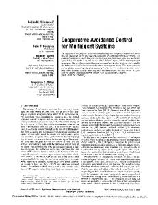

![([PDF]) Software Failure: Management Failure - Google Sites](https://m.moam.info/img/260x300/pdf-software-failure-management-failure-google-sit_6478835a097c4786708ce84f.jpg)