Behavior Research Methods 2009, 41 (4), 1111-1120 doi:10.3758/BRM.41.4.1111
BayesGCM: Software for Bayesian inference with the generalized context model Wolf Vanpaemel
University of Leuven, Leuven, Belgium This article describes and demonstrates the BayesGCM software package. The software is designed to perform Bayesian analysis with the generalized context model (GCM). It is intended to make the GCM easily accessible to a general public of experimental, social, and clinical psychologists interested in category learning, sensitivity, and attention. The software uses MATLAB and relies on WinBUGS to draw samples from the posterior distribution of the GCM’s parameters. The returned output comprises the full set of posterior samples, summary descriptive statistics, and graphs of the posterior distribution for each parameter of interest.
The software package described in this article, BayesGCM, involves Nosofsky’s (1986) generalized context model (GCM). The GCM is a highly influential model of category learning, built around two critical assumptions. The first assumption is that learning a category involves storing all individual category examples (exemplars) in memory. A categorization decision is then based on similarity comparisons with the stored exemplars. The second cornerstone of the GCM is that these similarities are subject to the operation of selective attention processes. The software relies on Bayesian methods to make inferences about the free parameters of the GCM, which include a measure of the ability to discriminate distinct exemplars in memory (the sensitivity), a measure of the attention given to a stimulus dimension, and two measures relating to people’s response behavior: the bias and the amount of determinism. Using Process Models As Measurement Models There seems to be a natural evolution in which a cognitive process model that has successfully passed a wide array of empirical tests comes to be used as a measurement model. When a model is used as a measurement model, confronting the model with data no longer has the goal of testing hypotheses about a particular cognitive process, as formalized by the model. Rather, the intention is to test hypotheses about parameter values. In this sense, the model serves as a statistical tool, much as, for example, the general linear model is used to test hypotheses about differences between groups. Consider, for example, multidimensional scaling (MDS). Originally, it was proposed as a model of human conceptual structure and generalization (Shepard, 1957, 1987). Nowadays, however, it is widely employed to generate a meaningful geometric representation of a set of stimuli. In this sense, the main interest is in the values
of the free parameters, which correspond to the coordinates. The use of MDS as a measurement model has found wide application in psychometrics, cognitive science, and psychophysics (Carrasco & Ridout, 1993; Hollins, Faldowski, Rao, & Young, 1993). Furthermore, MDS is a major research tool in financing and marketing, where it is known as perceptual mapping (Cooper, 1983; Frances & Groenen, 2000; P. Green, 1975). Similarly, there exists an interesting equivalence between the fuzzy logical model of perception (FLMP; e.g., Oden & Massaro, 1978) and the Rasch model. The FLMP is a widely applied process model of information integration, providing a psychological account of how people merge potentially ambiguous or conflicting information from various sensorial sources or modalities (e.g., auditory and visual). The Rasch model, on the other hand, is a dominant measurement model in psychometrics, commonly used to measure abilities, attitudes, and traits. Crowther, Batchelder, and Hu (1995) have shown that the FLMP can be rewritten as the Rasch model, thereby suggesting the potential applicability of the FLMP as a measurement model. Finally, models based on signal detection theory (SDT; e.g., D. Green & Swets, 1966) provide a theoretically based, detailed processing account of how people make decisions. In addition, researchers frequently use these models to measure discriminability and bias in people’s responses in detection tasks. The practice of using cognitive models as measurement tools has been termed cognitive psychometrics (Batchelder, 1998; Riefer, Knapp, Batchelder, Bamber, & Manifold, 2002). Cognitive psychometrics has important applicability to many psychological assessment problems, most notably in clinical cognitive science (McFall & Townsend, 1998; Neufeld, 2002, 2007; Treat & Dirks, 2007), where cognitive process models are used as assess-
W. Vanpaemel,
[email protected]
1111
© 2009 The Psychonomic Society, Inc.
1112 Vanpaemel ment tools to measure cognitive deficits in clinical populations. During the last decade, this field has witnessed an impressive growth (see, e.g., Busemeyer & Stout, 2002; Carter & Neufeld, 1999; Chechile, in press; Filoteo & Maddox, 1999; Knight & Silverstein, 2001). Using the GCM As a Measurement Model To be acceptable as a measurement model, a process model must satisfy a number of basic conditions. First, the model should have passed a wide array of empirical tests. The two theoretical claims of the GCM have been thoroughly tested against empirical data. First, investigating whether categories are represented by exemplars, rather than by an abstracted prototype, typically involves comparing the GCM with a prototype model, such as the MDS-based prototype model (MPM; Reed, 1972) on its ability to account for the empirical data (see Nosofsky, 1992, for an overview of GCM vs. MPM comparisons). Second, in an effort to find out whether or not category learning involves selective attention, the GCM has often been contrasted to decision bound models (Ashby & Gott, 1988) with respect to empirical data (see Ashby & Lee, 1991, 1992; Maddox & Ashby, 1998; McKinley & Nosofsky, 1996; Nosofsky, 1998; Nosofsky & J. E. Smith, 1992, for a series of exchanges on this topic). The overall picture that emerges is that the GCM provides excellent accounts of empirical data across an impressive array of experimental conditions. A second requirement concerns the model’s parameters. Not only should the parameters be identifiable (i.e., it should be possible to find estimates that are unique) and have a psychologically useful and interesting interpretation, they should also be shown to represent the cognitive processes that they are assumed to be associated with. In other words, it is essential to provide evidence that it is warranted to interpret the parameters as valid measures of their corresponding cognitive constructs. Establishing validity typically involves demonstrating that an experimental manipulation has a strong, predictable, and selective influence on the parameters. A second source of validity is the demonstration that parameter estimates map meaningfully onto independently provided measures. The GCM has passed several of such validity tests. For example, it has been shown that dimensional attention is affected in a predictable and theoretically interpretable way by variables such as category structure (e.g., Nosofsky, 1986, 1987, 1989) and time pressure (Lamberts, 1995). Similarly, sensitivity has been demonstrated to be affected in a psychologically meaningful way by time pressure (Lamberts, 1995) and by the number of training trials (J. D. Smith & Minda, 1998). Furthermore, it has been shown to be smaller for amnesics than for controls (Nosofsky & Zaki, 1998). The successful empirical and validity tests of the GCM and the identifiability and interpretability of its parameters speak well for the usefulness of the GCM as a measurement tool for constructs such as sensitivity and dimensional attention. From this perspective, modeling data using the GCM does not aim at evaluating a particular
theory about category representation or about selective attention processes but, rather, attempts to extract, through the GCM’s free parameters, meaningful information from the data that is not directly observable. In its capacity as a measurement tool, the usefulness of the GCM is not restricted to category learning research. Since attention is a crucial construct of interest across many fields of psychology (e.g., Franken, 2003; MacLeod, Mathews, & Tata, 1986; Mogg, Bradley, & Williams, 1995), estimates of attention weights are potentially highly informative for more applied researchers. For example, in an attempt to assess whether bulimics pay more attention to body size than nonbulimics do, Viken, Treat, Nosofsky, McFall, and Palmeri (2002) set up a prototype categorization task and analyzed the observed data using the MPM, which, like the GCM, incorporates free parameters corresponding to attention weights. Consistent with the expectations, it was found that bulimic women showed greater attention than did controls to body size and less attention to affect. Also the sensitivity parameter can provide insights relevant for applied research. For example, Bott, Brock, Brockdorff, Boucher, and Lamberts (2006) compared estimates of the sensitivity parameter to investigate whether highfunctioning adults with autism have a reduced sense of similarity, relative to nonautistic controls. Their analyses did not support this hypothesis. In sum, the GCM is a simple model with identifiable, useful, and easy-to-understand parameters that has successfully passed a wide variety of empirical and validity tests. Therefore, it seems well suited to being used as a measurement tool in cognitive psychometrics to provide clinically relevant information. The BayesGCM package described in this article provides an easy-to-use tool to exactly extract this kind of information. Bayesian Inference As its name suggests, the BayesGCM software package relies on Bayesian methods for statistical inference (e.g., Gelman, Carlin, Stern, & Rubin, 2004; Jaynes, 2003). As in most empirical sciences, Bayesian methods are rapidly being recognized as the most complete and coherent available way to relate models and data in psychology (e.g., Kuss, Jäkel, & Wichmann, 2005; Lee, 2008b; Lee & Wagenmakers, 2005; Myung & Pitt, 1997; Rouder & Lu, 2005), but to date, the number of applications of Bayesian methods in psychology remains somewhat limited. Perhaps the most important reason Bayesian methods have resisted widespread application is the relative high degree of technical sophistication required to perform a Bayesian analysis. Recently, this hindrance has started to diminish by virtue of the availability of well-documented tutorials on Bayesian methods (e.g., Wetzels, Lee, & Wagenmakers, 2009) and easy-to-use software packages for Bayesian analysis (e.g., the BayesSDT package for performing Bayesian analysis using SDT; Lee, 2008a). The BayesGCM package does not require a background in mathematics or any advanced programming language experience. Therefore, it represents another step in mak-
BayesGCM 1113 ing Bayesian methods available to a general audience, thereby promoting the use of model-based analyses in applied domains. In what follows, we will formally describe the GCM and discuss the theoretical and technical background to Bayesian methods. We then will present the BayesGCM software and an illustrative example of its use and its outputs. The Generalized Context Model Category Learning Task A typical category learning task involves a small set of simple perceptual stimuli varying along two salient dimensions and two categories to be learned. These categories are created by assigning a subset of the stimuli to Category A and another subset to Category B. Often, it also involves a number of unassigned stimuli. In most tasks, the training–test procedure is used, which consists of a training phase followed by a test phase. During the training phase, the category structure is learned. Each assigned stimulus is presented to and classified by the participant into either Category A or B. Following each response, corrective feedback is presented, which can be either deterministic or probabilistic, depending on whether or not the stimulus receives the same feedback every time it is presented. During the test phase, both the assigned and the unassigned stimuli are presented. Generally, corrective trial-by-trial feedback continues to be provided on trials in which assigned stimuli are presented but is withheld on trials in which unassigned stimuli are presented, because there are no correct or incorrect answers for these trials. The relevant data for modeling are the categorization decisions from the test phase—that is, for each stimulus, the number of times it was chosen in Category A out of the total number of trials on which it was presented during the test phase. The Generalized Context Model The GCM assumes that stimuli are represented as points in a multidimensional psychological space. This geometric stimulus representation is typically derived using MDS (Kruskal, 1964), on the basis of pairwise similarities obtained from a similarity rating task. Let xi 5 (xi1,xi2) denote the coordinate locations of stimulus xi in a 2-D space. Given the coordinates of the stimuli, the distance between stimuli xi and xj is computed according to the Minkowski metric:
(
)
1/ r
d xi , x j = w | xi1 − x j1 |r + (1 − w ) | xi 2 − x j 2 | r , (1) where r is the metric and w is the attention weight parameter. Most often, r is not considered a free parameter but is assumed to depend on the type of dimensions that compose the stimuli. Generally, the city block metric (r 5 1) is used when stimuli vary on separable dimensions, and the Euclidean metric (r 5 2) is used for stimuli varying on integral dimensions (see Shepard, 1991, for a review).
The attention weight w models the psychological process of selective attention. It corresponds to the salience of the first dimension, or the relative attention given to the first dimension over the second. The underlying motivation for this parameter is the idea that people who are faced with a categorization task are inclined to focus on the dimensions that are relevant for the categorization task at hand and to ignore the dimensions that are irrelevant. Similarity is then modeled as a decaying function of the distance between the stimuli:
(
{
)
(
s xi , x j = exp − cd xi , x j
)
α
}
,
(2)
where α determines the shape of the function and c is the sensitivity parameter. Much as with the metric parameter r, α is not considered a free parameter but depends on the nature of the stimuli. Generally, when stimuli are readily discriminable, the exponential decay function (α 5 1) seems to be the appropriate choice, whereas the Gaussian function (α 5 2) is typically preferred when the stimuli are highly confusable (Shepard, 1987). The sensitivity parameter c corresponds to the rate at which similarity declines with distance. A high value of c implies that only stimuli that lie very close to each other are considered as being similar, whereas a low value of c implies that all the stimuli are at least somewhat similar to each other. These similarities are used to compute the similarity between a stimulus and a category. Being an exemplar model, the GCM assumes that a category is represented by all its members: and
s ( xi , A ) =
∑ a j Nj j
(
(
)
)
(
s xi , x j ,
)
s ( xi , B ) = ∑ 1 − a j Nj s xi , xj . (3) j The variable aj represents the probability with which stimulus xi receives Category A feedback. If feedback is deterministic, aj only takes on the values zero or one: If stimulus xj belongs to Category A, then aj 5 1, and aj 5 0 otherwise. The variable Nj represents the frequency with which stimulus xi is presented during training. The product of aj and Nj is sometimes referred to as the memory strength of stimulus xi . The more often and the more consistently a stimulus has been presented as a member of a category, the greater its memory strength. The response probability for stimulus xi ’s being chosen as a member of Category A is computed according to the choice rule: pi = p ( A | xi ) =
β s ( xi , A )
γ
β s ( xi , A ) + (1 − β ) s ( xi , B ) γ
γ
. (4)
This expression includes two additional free parameters: the bias parameter β, which reflects any response bias to Category A, and the response-scaling parameter γ (Ashby & Maddox, 1993; Navarro, 2007), which reflects the
1114 Vanpaemel amount of determinism in responding. A high value of γ implies that a stimulus that is more similar to Category A than to Category B tends to be classified in Category A, whereas a low value of γ implies that such a stimulus is sometimes classified in Category B. Finally, it is assumed that, for each stimulus presented in the test phase, the counts follow a binomial distribution. If ti denotes the number of times stimulus xi was presented in the test phase and ki the number of times stimulus xi was assigned to Category A, the likelihood is given by
ki ~ Binomial( pi ,ti ).
(5)
Parameter Priors Application of Bayesian methods requires specifying a prior distribution for each of the free parameters involved, which expresses the belief, before the data are collected, as to which values of the parameters are likely and unlikely. On the basis of experience with previous related studies, or on theoretical grounds, a researcher can have a priori reasons to believe that some values are more likely than others. This information can be translated in an informative prior. In the absence of such information, an uninformative prior is more apt, which is intended to reflect a state of ignorance by not favoring any parameter values over others. The priors used in the current version of BayesGCM are all noninformative. In particular, BayesGCM assumes the following priors: The attention weight w and the bias β are given a uniform prior distribution over the interval between zero and one:
w ~ Uniform(0,1),
(6)
β ~ Uniform(0,1).
(7)
Similarly, the response determinism γ is given a uniform prior distribution over the interval between zero and 20:
γ ~ Uniform(0,20).
(8)
Finally, as far as the sensitivity c is concerned, it is useful to note that 1/c scales the distances (see Equation 2); hence, c functions as an inverse scale, implying that c2 functions as a precision. The standard (near) noninformative prior distribution for the precision is given by (see Spiegelhalter, Thomas, Best, Gilks, & Lunn, 1994)
c2 ~ Gamma(ε,ε),
(9)
with ε 5 .001 set near zero. This prior has the attractive property that it makes inferences about the c parameter (nearly) invariant to the scale on which distances are measured (see Jaynes, 2003, chaps. 12 and 13, for a detailed discussion). It should be noted that different choices of a prior can lead to different results as far as model selection is concerned, whereas parameter estimation is generally relatively robust to the specific shape of the prior. If enough observations are made, the data overwhelm the prior, so the exact choice of the prior does not greatly affect inference.
Bayesian Inference, Sampling, and Graphical Models Bayesian Inference The Bayesian approach to parameter estimation is to use a probability distribution over the parameters, which contains all the available information. The main interest is in the posterior distribution, which specifies the relative probability that each possible combination of parameter values is the one that generated the observed behavior. In particular, BayesGCM generates the marginal posterior distribution of each parameter, conditional on the observed data. Bayesian methods contrast favorably with standard methods in the context of inferring parameters from data. First, Bayesian methods are sensitive to how many data are available and are automatically exact for any sample size. Second, the posterior distribution over a parameter contains more information than does a single point estimate, in the sense that the distribution not only indicates which parameter values are probable, but also shows the uncertainty about those values. Finally, it is worth noting that the posterior distribution is not constrained to take a particular parametric form but, instead, is free to take the form that follows from the specification of the model and from the information provided by data. Posterior Sampling For most cognitive models, it is impossible to find analytic expressions for the posterior distribution. Instead, modern Bayesian inference proceeds computationally by drawing samples from the posterior distribution. Sampling from a distribution relies on the fact that, over a large number of samples, the relative probability of a particular combination of parameter values in the distribution is approximated by the relative frequency of those values. This correspondence allows approximating the information present in the exact distribution by simple computations across the samples. For example, the distribution of a variable is approximated by the histogram of the sampled values, and the expected value is approximated by the arithmetic average over the sampled values. For sampling, the BayesGCM package relies on WinBUGS (Sheu & O’Curry, 1998; Spiegelhalter, Thomas, Best, & Lunn, 2004), which uses a range of Markov chain Monte Carlo computational methods to perform sampling (see, e.g., Chen, Shao, & Ibrahim, 2000; Gamerman & Lopes, 2006; Gilks, Richardson, & Spiegelhalter, 1996). A number of excellent worked-out examples of how psychologists can benefit from WinBUGS are provided by Lee (2008b) and Shiffrin, Lee, Wagenmakers, and Kim (2008). Graphical Models Implementing a model in WinBUGS is greatly facilitated by expressing the model as a graphical model (see Griffiths, Kemp, & Tenenbaum, 2008, and Lee, 2008b, for psychological introductions; see Jordan, 2004, and
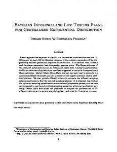
BayesGCM 1115 Koller, Friedman, Getoor, & Taskar, 2007, for statistical introductions). In graphical modeling, a graph is created in which nodes represent the variables of interest. The graph structure indicates dependencies between the variables, with arrows indicating the direction of the dependency. Figure 1 presents a graphical model interpretation of the GCM, using the following conventions. Continuous variables are shown with circular nodes, and discrete variables are shown with square nodes. Observed variables (i.e., the data and the variables making up the experimental design) are shown with shading, and unobserved variables (including the parameters to be inferred from the data) are shown without shading. Stochastic variables are shown with single borders, and deterministic variables are shown with double borders. Independent replications in the model are indicated by square plates.
l = 1, . . . , m ∪ n k = 1, 2
j = 1, . . . , n
w
dij
r
c
sij
α
i = 1, . . . , m j = 1, . . . , n pi
aj
j = 1, . . . , n γ
ki
ti
The BayesGCM software package can be downloaded from http://ppw.kuleuven.be/concat. It consists of four MATLAB functions (.m files) and one WinBUGS script (.txt file). The BayesGCM user needs only to directly call one MATLAB function, BayesGCM.m, which calls the other MATLAB functions and the WinBUGS script when necessary. The package also contains an additional MATLAB script, BayesGCM_demo.m, which is not necessary for the correct functioning of the package but provides a detailed example of how to declare the data and run the code. Using BayesGCM requires MATLAB (The MathWorks, Inc., 2007) and WinBUGS (1.4.2 or later) to be installed. WinBUGS is available at no cost from www.mrc-bsu.cam .ac.uk/bugs/winbugs/contents.shtml. For passing information between MATLAB and WinBUGS, BayesGCM relies on the matbugs.m MATLAB function, which is freely available at www.cs.ubc.ca/~murphyk/Software/ MATBUGS/matbugs.html. Use The BayesGCM software provides a MATLAB function call to use WinBUGS, using the following simple syntax: [samples stats] 5 BayesGCM(D). The input D and the output samples and stats will be discussed below, as well as other forms of output.
xlk
β
The BayesGCM Software Package
Nj
i = 1, . . . , m Figure 1. Graphical model interpretation of the generalized context model for inferring attention (w), sensitivity (c), bias (β), and response determinism (γ) from ki observed Category A classifications out of ti stimulus presentations, with n assigned stimuli and m stimuli presented in the test phase.
Input The input is organized using a structured variable D with 22 fields. Table 1 gives a schematic overview of the required inputs. A specific example of how this structured variable should be declared is provided by the MATLAB script BayesGCM_demo.m. Bookkeeping. BayesGCM requires specifying the number of data sets to be analyzed, a label for each data set, and a location and a name to save the output. The version of the GCM. BayesGCM allows for considerable flexibility as to which exact version of the GCM should be applied. The BayesGCM user can specify whether or not the w, β, and γ parameters should be included. Experimental design. BayesGCM needs several variables that specify the experimental design. First, it needs the 2-D geometric representation of all the stimuli, the metric, and the similarity gradient. Furthermore, it needs a vector indicating the probability with which each stimulus is assigned to Category A (21 if unassigned), a vector indicating the number of times each stimulus was presented during the training phase (0 if not presented), and a vector indicating the number of times each stimulus was presented during the test phase (0 if not presented). Empirical data. The observed data take the form of counts, representing, for each stimulus, the number of times it was classified as belonging to Category A (0 if not presented). Sampling variables. It is good practice to check for convergence using multiple independent runs (chains).
1116 Vanpaemel Table 1 Notation and Content for the Input Required by BayesGCM Field D.ndatasets D.labels D.name D.loc D.wcheck D.bcheck D.gcheck D.c D.r D.a D.f D.N D.t D.k D.nchains D.nburnin D.nsamples D.nbins D.linewidth D.linecolor D.linestyle D.rcheck
Content the number of data sets to be analyzed cell array containing, for each data set, a character array with the label to use in the output character array with the name to save the output character array with the location to save the output vector indicating, for each data set, whether (1) or not (0) the w parameter should be included in the GCM vector indicating, for each data set, whether (1) or not (0) the β parameter should be included in the GCM vector indicating, for each data set, whether (1) or not (0) the γ parameter should be included in the GCM cell array containing, for each data set, the matrix with the 2-D coordinates of the stimuli vector of 1 and 2 entries indicating, for each data set, the metric vector of 1 and 2 entries indicating, for each data set, the similarity gradient cell array containing, for each data set, a vector with the probability that a stimulus received Category A feedback (21 for unassigned stimulus) cell array containing, for each data set, a vector with the number of times each stimulus was presented in the training phase (0 for unpresented stimulus) cell array containing, for each data set, a vector with the number of times each stimulus was presented in the test phase (0 for unpresented stimulus) cell array containing, for each data set, a vector with the number of times each stimulus was classified in Category A (0 for unpresented stimulus) the number of independent runs using the same data set the number of posterior samples at the beginning of a sampling run that are not recorded the number of posterior samples to generate and record the number of bins to use in drawing histograms of the posterior densities vector with, for each data set, a line width to use in drawing the graphs character array with, for each data set, a color to use in drawing the graphs, using the standard MATLAB plot colors character array with, for each data set, a line style to use in drawing the graphs, using the standard MATLAB line styles vector indicating, for each data set, whether (1) or not (0) the proportion of variance accounted for should be calculated using the mean parameter values only
Therefore, the BayesGCM user needs to specify the number of chains to be run. Furthermore, BayesGCM needs the number of posterior samples to be generated in each chain (including burn-in samples—i.e., samples that are not recorded). Including additional samples increases the computing time but results in a better approximation to the posterior distribution. Output variables. To display the posterior densities, the BayesGCM user needs to specify the number of bins, as well as the width, color, and style properties of the lines used to draw the posterior distribution for each data set, using standard MATLAB options. Finally, BayesGCM calculates the proportion of variance accounted for (r 2) on the basis of each (recorded) posterior sample. However, since this calculation might take a long time when the number of samples is large, it is possible to indicate that r 2 should be calculated only on the basis of the mean parameter value. Output The main result of the analysis is a graphical output. For each of the analyzed parameters, BayesGCM generates a graph of the posterior distributions. BayesGCM also generates a MATLAB mat file, ending with _samples&stats .mat, containing the input and two structured variables returned by WinBUGS, samples and stats. The fields in samples provide, for each data set, the full list of posterior samples of each analyzed parameter. On the basis of the samples, all relevant statistics can be easily calculated, two of which are automatically provided in stats. In particular, the fields in stats provide, for each data set, the
means and standard deviations for the posterior samples of each analyzed parameter. When multiple chains are run, stats also provides, for each data set and for each parameter, a quantitative measure for diagnosing convergence. The statistic, provided in stats.Rhat, compares within- to between-chain variability. A value less than 1.1 indicates that the chain has probably converged (Gelman & Rubin, 1992). Finally, BayesGCM generates a text file, ending with _summary.txt, listing, for each data set and for each of the parameters of interest, the mean, the median, the mode, the standard deviation, and, if applicable, the convergence diagnostic Rhat. Furthermore, the summary text file also displays, for each data set, the proportion of variance accounted for and the time used for sampling. Demonstration We will demonstrate BayesGCM using two illustrative data sets taken from an influential study by Nosofsky (1989). The MATLAB script BayesGCM_demo.m contains all relevant input and syntax to do the analysis presented here. Nosofsky’s (1989) experiment involved a set of 16 semicircles with an embedded radial line drawn from the center of the semicircle to the rim. The stimuli varied in the size of the semicircle and in the angle of orientation of the line. Using data from an identification experiment, Nosofsky (1989) derived a 2-D representation of the stimulus space. On the basis of this set of 16 stimuli, Nosofsky (1989) defined four different category structures. Two of these structures, the angle and the size structures, are of
BayesGCM 1117 Angle 13
9
Size 14
15
10
11
6
5
1
2
7
16
9
12
4
14
15
10
11
6
5
8
3
13
1
2
7
16
12
8
3
4
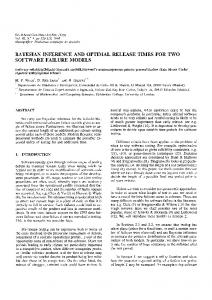
Figure 2. The angle and size category structures from Nosofsky (1989). Squares denote stimuli assigned to Category A, and circles denote stimuli assigned to Category B. The remaining stimuli are unassigned. The horizontal dimension corresponds to angle, and the vertical dimension to size. Both structures require attending to a single dimension only to learn the categories.
particular interest for demonstrating the BayesGCM package, since they are used to investigate selective attention processes in category learning. They are shown schematically in Figure 2. The dimension on the horizontal axis corresponds to the angle, and the vertical axis corresponds to the size. As is clear from Figure 2, attending one dimension only is sufficient to learn the category structures. In the angle structure (panel A), stimuli with low angles are assigned to Category A, and stimuli with high angles are assigned to Category B. In the size structure (panel B), small stimuli are assigned to Category A, and large stimuli are assigned to Category B. Each category structure was learned by a separate group of participants under the training–test procedure. During the training phase, each stimulus was presented with equal frequency and received deterministic feedback. During the test phase, each unassigned stimulus was presented twice, and each assigned stimulus was presented approximately six times. Nosofsky (1989) restricted the modeling analyses to those participants who, on average, classified the assigned stimuli with 70% and 80% accuracy or better during the final 125 training trials in the angle and size conditions, respectively. This criterion was met by 41 of 83 and 37 of 44 participants in each respective condition. To illustrate how Bayesian analysis represents the decrease in uncertainty with additional data, we constructed two toy data sets using the angle and size category structures. These toy data sets were created by multiplying or dividing the number of test trials and the number of observed responses by 50, resulting in two data sets in which the response pattern was identical to the response pattern actually observed by Nosofsky (1989), but the sample size (i.e., the number of observations per stimulus) was either much larger or much smaller. Each data set was analyzed using the baseline version of the GCM, which includes the sensitivity c and the at-
tention w but excludes the bias β and the response determinism γ. Three chains were run of 105 samples each after a 103-sample burn-in period. The stats.Rhat statistics were all very close to 1, suggesting convergence, so the samples were collapsed across the three chains. Sampling three chains took, on average, 11 min for a single data set, on a PC with a processor speed of 3 GHz and 1 Gb of RAM. Figure 3 shows the graphical output of the BayesGCM software, for the small sample size data, the observed data, and the large sample size data. It shows the posterior distribution over the sensitivity and over the attention given to the angle dimension, using 100 bins. The attention given to the size dimension is simply one minus the attention given to the angle dimension. The posterior distributions give a natural visual representation of the uncertainty about the parameter values. The posterior distributions for the large sample size data set, shown on the right, show that the parameters are estimated with relatively little uncertainty. The posterior distributions for the small sample size data set, shown on the left, show a much greater degree of uncertainty. The posteriors for the actually observed data are somewhere in between with respect to uncertainty. This clearly shows the intuitive effect of increasing the sample size: Observing more data naturally leads to a reduction in uncertainty. For the present demonstration, we are mostly interested in the attention weights, shown in the second row of Figure 3. Even when sample size is small, there is a clear difference in the attentional distribution across both structures. For the angle structure, the mode of the posterior distribution of the attention weight is close to 1, whereas the mode of the posterior distribution of the attention weight for the size structure is close to 0. However, the range of likely parameter values is not heavily restricted. On the basis of little data, it is still possible for the attentional distribution to be the other way around.
1118 Vanpaemel
A
B
C
0
5
10
15
20
25
Posterior Density
Posterior Density
Posterior Density
Angle Size
0
1
2
3
4
0.6
0.8
1
3
4
Posterior Density
F
Posterior Density 0.4
Attention (w)
2
Sensitivity (c)
E
Posterior Density
D
0.2
1
Sensitivity (c)
Sensitivity (c)
0
0
0
0.2
0.4
0.6
Attention (w)
0.8
1
0
0.2
0.4
0.6
0.8
1
Attention (w)
Figure 3. Posterior distributions for sensitivity (c, first row) and attention to the angle dimension (w, second row) for Nosofsky’s (1989) angle and size category structures, using a small (panels A and D), the empirical (panels B and E), and a large (panels C and F) sample size.
Much firmer conclusions are possible given the observed data and the large sample size data. As was expected and reported by Nosofsky (1989), the posterior distributions show clearly that the participants attended selectively to the angle dimension when learning the angle category structure and gave greater weight to the size dimension when learning the size category structure. Conclusion This article has described and demonstrated the BayesGCM software package, which can be used for performing Bayesian parameter estimation in the GCM. BayesGCM is relatively easy to use and requires no advanced MATLAB or WinBUGS experience. For each parameter analyzed, BayesGCM returns a graph of the posterior distribution. Using the GCM to analyze data collected in a category learning task affords insights in sensitivity, attention, bias, and response determinism, corresponding to the free parameters of the GCM. Probably the psychologically most
interesting free parameters are the sensitivity, corresponding to people’s ability to discriminate distinct exemplars in memory, and the attention weights, reflecting how people distribute their attention over dimensions. Since sensitivity and attention are important variables across many fields, the usefulness of BayesGCM goes beyond category learning research, stretching to clinical, social, health, and personality psychology. Author Note This work was funded by Grant FWO G.0513.08. I thank Laurence Claes, Gert Storms, Rob Nosofsky, and Michael Lee for their valuable suggestions. Correspondence concerning this article should be addressed to W. Vanpaemel, Department of Psychology, University of Leuven, Concat, Tiensestraat 102, B-3000 Leuven, Belgium (e-mail: wolf.vanpaemel@ psy.kuleuven.be; Web site: http://ppw.kuleuven.be/concat). References Ashby, F. G., & Gott, R. E. (1988). Decision rules in the perception and categorization of multidimensional stimuli. Journal of Experimental Psychology: Learning, Memory, & Cognition, 14, 33-53.
BayesGCM 1119 Ashby, F. G., & Lee, W. W. (1991). Predicting similarity and categorization from identification. Journal of Experimental Psychology: General, 120, 150-172. Ashby, F. G., & Lee, W. W. (1992). On the relationship among identification, similarity, and categorization: Reply to Nosofsky and Smith (1992). Journal of Experimental Psychology: General, 121, 385-393. Ashby, F. G., & Maddox, W. T. (1993). Relations between prototype, exemplar, and decision bound models of categorization. Journal of Mathematical Psychology, 37, 372-400. Batchelder, W. H. (1998). Multinomial processing tree models and psychological assessment. Psychological Assessment, 10, 331-344. Bott, L., Brock, J., Brockdorff, N., Boucher, J., & Lamberts, K. (2006). Perceptual similarity in autism. Quarterly Journal of Experimental Psychology, 59A, 1237-1254. Busemeyer, J. R., & Stout, J. C. (2002). A contribution of cognitive decision models to clinical assessment: Decomposing performance on the Bechara gambling task. Psychological Assessment, 14, 253-262. Carrasco, M., & Ridout, J. B. (1993). Olfactory perception and olfactory imagery: A multidimensional analysis. Journal of Experimental Psychology: Human Perception & Performance, 19, 287-301. Carter, J. R., & Neufeld, R. W. J. (1999). Cognitive processing of multidimensional processing in schizophrenia: Formal modeling of judgment speed and content. Journal of Abnormal Psychology, 108, 633-654. Chechile, R. A. (in press). Modeling storage and retrieval processes with clinical populations with applications examining alcoholinduced amnesia and Korsakoff amnesia. Journal of Mathematical Psychology. Chen, M. H., Shao, Q. M., & Ibrahim, J. G. (2000). Monte Carlo methods in Bayesian computation. New York: Springer. Cooper, L. G. (1983). A review of multidimensional scaling in marketing research. Applied Psychological Measurement, 7, 427-450. Crowther, C. S., Batchelder, W. H., & Hu, X. (1995). A measurementtheoretic analysis of the fuzzy logic model of perception. Psychological Review, 102, 396-408. Filoteo, J. V., & Maddox, W. T. (1999). Quantitative modeling of visual attention processes in patients with Parkinson’s disease: Effects of stimulus integrality on selective attention and dimensional integration. Neuropsychology, 13, 206-222. Frances, P. H., & Groenen, P. (2000). Visualizing time-varying correlations across stock markets. Journal of Empirical Finance, 7, 155-172. Franken, I. (2003). Drug craving and addiction: Integrating psychological and neuropsychopharmacological approaches. Progress in NeuroPsychopharmacology & Biological Psychiatry, 27, 563-579. Gamerman, D., & Lopes, H. F. (2006). Markov chain Monte Carlo: Stochastic simulation for Bayesian inference. Boca Raton, FL: Chapman & Hall/CRC. Gelman, A., Carlin, J. B., Stern, H. S., & Rubin, D. B. (2004). Bayesian data analysis. London: Chapman & Hall. Gelman, A., & Rubin, D. B. (1992). Inference from iterative simulation using multiple sequences. Statistical Science, 7, 457-472. Gilks, W., Richardson, S., & Spiegelhalter, D. J. (Eds.) (1996). Markov chain Monte Carlo in practice. Suffolk, U.K.: Chapman & Hall. Green, D., & Swets, J. (1966). Signal detection theory and psychophysics. New York: Wiley. Green, P. (1975). Marketing applications of MDS: Assessment and outlook. Journal of Marketing, 39, 24-31. Griffiths, T. L., Kemp, C., & Tenenbaum, J. B. (2008). Bayesian models of cognition. In R. Sun (Ed.), Cambridge handbook of computational cognitive modeling (pp. 59-100). Cambridge: Cambridge University Press. Hollins, M., Faldowski, R., Rao, S., & Young, F. (1993). Perceptual dimensions of tactile surface texture: A multidimensional scaling analysis. Perception & Psychophysics, 54, 697-705. Jaynes, E. T. (2003). Probability theory: The logic of science. New York: Cambridge University Press. Jordan, M. I. (2004). Graphical models. Statistical Science, 19, 140155. Knight, R. A., & Silverstein, S. M. (2001). A process-oriented approach for averting confounds resulting from general performance deficiencies in schizophrenia. Journal of Abnormal Psychology, 110, 15-30.
Koller, D., Friedman, N., Getoor, L., & Taskar, B. (2007). Graphical models in a nutshell. In L. Getoor & B. Taskar (Eds.), Introduction to statistical relational learning (pp. 13-55). Cambridge, MA: MIT Press. Kruskal, J. (1964). Multidimensional scaling by optimizing goodness of fit to a nonmetric hypothesis. Psychometrika, 29, 1-27. Kuss, M., Jäkel, F., & Wichmann, F. A. (2005). Bayesian inference for psychometric functions. Journal of Vision, 5, 478-492. Lamberts, K. (1995). Categorization under time pressure. Journal of Experimental Psychology: General, 124, 161-180. Lee, M. D. (2008a). BayesSDT: Software for Bayesian inference with signal detection theory. Behavior Research Methods, 40, 450-456. Lee, M. D. (2008b). Three case studies in the Bayesian analysis of cognitive models. Psychonomic Bulletin & Review, 15, 1-15. Lee, M. D., & Wagenmakers, E. J. (2005). Bayesian statistical inference in psychology: Comment on Trafimow (2003). Psychological Review, 112, 662-668. MacLeod, C., Mathews, A., & Tata, P. (1986). Attentional bias in emotional disorders. Journal of Abnormal Psychology, 95, 15-20. Maddox, W. T., & Ashby, F. G. (1998). Selective attention and the formation of linear decision boundaries: Comment on McKinley and Nosofsky (1996). Journal of Experimental Psychology: Human Perception & Performance, 24, 301-321. The MathWorks, Inc. (2007). MATLAB—The language of technical computing, Version 7.5 [Computer software manual]. Natick, MA. Available at www.MathWorks.com/products/matlab/. McFall, R. M., & Townsend, J. T. (1998). Foundations of psychological assessment: Implications for cognitive assessment in clinical science. Psychological Assessment, 10, 316-330. McKinley, S. C., & Nosofsky, R. M. (1996). Selective attention and the formation of linear decision boundaries. Journal of Experimental Psychology: Human Perception & Performance, 22, 294-317. Mogg, K., Bradley, B., & Williams, R. (1995). Attentional bias in anxiety and depression: The role of awareness. British Journal of Clinical Psychology, 34, 17-36. Myung, I. J., & Pitt, M. A. (1997). Applying Occam’s razor in modeling cognition: A Bayesian approach. Psychonomic Bulletin & Review, 4, 79-95. Navarro, D. J. (2007). On the interaction between exemplar-based concepts and a response scaling process. Journal of Mathematical Psychology, 51, 85-98. Neufeld, R. W. J. (2002). Introduction to the special section on cognitive science and psychological assessment. Psychological Assessment, 14, 235-238. Neufeld, R. W. J. (2007). Advances in clinical cognitive science: Formal modeling and assessment of processes and symptoms. Washington, DC: American Psychological Association. Nosofsky, R. M. (1986). Attention, similarity, and the identification– categorization relationship. Journal of Experimental Psychology: General, 115, 39-57. Nosofsky, R. M. (1987). Attention and learning processes in the identification and categorization of integral stimuli. Journal of Experimental Psychology: Learning, Memory, & Cognition, 13, 87-108. Nosofsky, R. M. (1989). Further tests of an exemplar-similarity approach to relating identification and categorization. Perception & Psychophysics, 45, 279-290. Nosofsky, R. M. (1992). Exemplars, prototypes, and similarity rules. In A. F. Healy, S. M. Kosslyn, & R. M. Shiffrin (Eds.), From learning theory to connectionist theory: Essays in honor of William K. Estes (Vol. 1, pp. 149-167). Hillsdale, NJ: Erlbaum. Nosofsky, R. M. (1998). Selective attention and the formation of linear decision boundaries: Reply to Maddox and Ashby (1998). Journal of Experimental Psychology: Human Perception & Performance, 24, 322-339. Nosofsky, R. M., & Smith, J. E. (1992). Similarity, identification, and categorization: Comment on Ashby and Lee (1991). Journal of Experimental Psychology: General, 121, 237-245. Nosofsky, R. M., & Zaki, S. R. (1998). Dissociations between categorization and recognition in amnesic and normal individuals: An exemplar-based interpretation. Psychological Science, 9, 247-255. Oden, G. C., & Massaro, D. W. (1978). Integration of featural information in speech perception. Psychological Review, 85, 172-191.
1120 Vanpaemel Reed, S. K. (1972). Pattern recognition and categorization. Cognitive Psychology, 3, 392-407. Riefer, D. M., Knapp, B. R., Batchelder, W. H., Bamber, D., & Manifold, V. (2002). Cognitive psychometrics: Assessing storage and retrieval deficits in special populations with multinomial processing tree models. Psychological Assessment, 14, 184-201. Rouder, J. N., & Lu, J. (2005). An introduction to Bayesian hierarchical models with an application in the theory of signal detection. Psychonomic Bulletin & Review, 12, 573-604. Shepard, R. N. (1957). Stimulus and response generalization: A stochastic model relating generalization to distance in psychological space. Psychometrika, 22, 325-345. Shepard, R. N. (1987). Toward a universal law of generalization for psychological science. Science, 237, 1317-1323. Shepard, R. N. (1991). Integrality versus separability of stimulus dimensions: From an early convergence of evidence to a proposed theoretical basis. In J. Pomerantz & G. Lockhead (Eds.), The perception of structure: Essays in honor of Wendell R. Garner (pp. 53-71). Washington, DC: American Psychological Association. Sheu, C.-F., & O’Curry, S. L. (1998). Simulation-based Bayesian inference using BUGS. Behavior Research Methods, Instruments, & Computers, 30, 232-237. Shiffrin, R. M., Lee, M. D., Wagenmakers, E.-J., & Kim, W.-J. (2008). A survey of model evaluation approaches with a focus on hierarchical Bayesian methods. Cognitive Science, 32, 1248-1284.
Smith, J. D., & Minda, J. P. (1998). Prototypes in the mist: The early epochs of category learning. Journal of Experimental Psychology: Learning, Memory, & Cognition, 24, 1411-1436. Spiegelhalter, D., Thomas, A., Best, N., Gilks, W., & Lunn, D. (1994). BUGS: Bayesian inference using Gibbs sampling. Cambridge: Medical Research Council Biostatistics Unit, Institute of Public Health. Available at www.mrc-bsu.cam.ac.uk/bugs. Spiegelhalter, D., Thomas, A., Best, N., & Lunn, D. (2004). WinBUGS User Manual Version 2.0. Cambridge: Medical Research Council Biostatistics Unit, Institute of Public Health. Treat, T. A., & Dirks, M. A. (2007). Bridging clinical and cognitive science. In T. A. Treat, R. R. Bootzin, & T. B. Baker (Eds.), Psychological clinical science: Papers in honor of Richard McFall. New York: Taylor & Francis. Viken, R., Treat, T., Nosofsky, R., McFall, R., & Palmeri, T. (2002). Modeling individual differences in perceptual and attentional processes related to bulimic symptoms. Journal of Abnormal Psychology, 111, 598-609. Wetzels, R., Lee, M. D., & Wagenmakers, E.-J. (2009). Bayesian inference using WBDev: A tutorial for social scientists. Manuscript submitted for publication. (Manuscript received July 20, 2008; revision accepted for publication June 6, 2009.)