IEEE TRANSACTIONS ON POWER SYSTEMS, VOL. 18, NO. 3, AUGUST 2003
1165
Software Implementation of Online Risk-Based Security Assessment Ming Ni, Member, IEEE, James D. McCalley, Senior Member, IEEE, Vijay Vittal, Fellow, IEEE, Scott Greene, Member, IEEE, Chee-Wooi Ten, Vijaya Sudhakar Ganugula, Member, IEEE, and Tayyib Tayyib, Member, IEEE
Abstract—This paper describes software implementation for online risk-based security assessment which computes indices based on probabilistic risk for use by operators in the control room to assess system security levels as a function of existing and near-future network conditions. The paper focuses on speed enhancement techniques that are essential for online application and result visualization methods that offer clear and meaningful ways to enhance human assimilation and comprehension of security levels. Results of testing on a series of 1600 bus power flow models retrieved from the energy management system of a large U.S. utility are presented and serve to illustrate the benefits of the software. Index Terms—Cascading, control center, decision-making, operations, overload, probabilistic risk, security assessment, uncertainty, visualization, voltage instability.
I. INTRODUCTION
T
HE power system has been shifting from a regulated system to a competitive and uncertain market environment, and the conditions under which power systems are operated have become more diverse. Transmission loading patterns differ from those for which they were originally planned, and the ability to monitor and control them has greatly increased in complexity. High uncertainty is a characterizing feature of this complexity. Although some methods of risk assessment and management have been introduced into the market-oriented energy trading business, traditional deterministic decision-making is still utilized within system operation. This has led engineers to face more pressure, from economic imperatives in the marketplace, to operate power systems with lower security margins, resulting in more frequent encounter with highly stressed conditions requiring operator decision. In response, a set of tools called risk-based security assessment (RBSA) [1]–[3] has been developed. An important feature of this approach is an index that quantitatively captures the basic factors that determine security level: likelihood and severity of events. Manuscript received July 17, 2002. This work was supported by the Electric Power Research Institute under Contract WO663101. M. Ni, J. D. McCalley and V. Vittal are with Iowa State University, Ames, IA 50010 USA (e-mail:
[email protected];
[email protected]; vvittal@ iastate.edu). S. Greene is with Pricewaterhousecoopers LLP, USA (e-mail:
[email protected]). C.-W. Ten is with Siemens Energy Management, Singapore (e-mail:
[email protected]). V. S. Ganugula is with ESCA, Bellevue, WA 98004 USA (e-mail: vijaya.
[email protected]). T. Tayyib is with the Electric Power Research Institute, Palo Alto, CA 94304 USA (e-mail:
[email protected]). Digital Object Identifier 10.1109/TPWRS.2003.814909
In [4], the concept of online risk-based security assessment (OL-RBSA) is proposed and developed which addresses control-room security-economy decision-making (CR/SE/DM). OL-RBSA computes indices based on probabilistic risk for the purpose of performing online security assessment of high voltage electric power transmission systems. The indices computed are for use by operators in the control room to assess system security levels as a function of existing and near-future network conditions. Uncertainties in near-future loading conditions and contingency conditions are modeled. Any number of contingencies may be included in the assessment. Severity functions are adopted to uniformly quantify the severity of network performance for overload and voltage security. The overload security indices include probabilistic expectations of the severity associated with high circuit flows and the severity associated with cascading overloads. The voltage security indices include probabilistic expectations of the severity associated with low bus voltages and the severity associated with voltage instability. High flows and low voltages are assessed with an ac power flow algorithm, and flow and voltage sensitivities with respect to uncertain operating parameters are computed. Cascading overloads are assessed with successive power flow solutions. Voltage instability is assessed with a continuation power flow method together with loadability sensitivities. Fig. 1 illustrates how OL-RBSA software is integrated with the existing SCADA/EMS system for control room application. In this paper, the software implementation of OL-RBSA is described. First, the software structure is introduced briefly in Section II. Because of restrictive run-time requirements associated with online security assessment applications, together with the inherent increased computational demands of analyzing uncertainty, analysis speed is a central issue in implementation of OL-RBSA. For that reason, we have used several approaches to enhance the computational efficiency. In addition, we have developed the program so that it can be easily run using any number of Pentium-based parallel processors running the Windows NT operating system, so that a large number of contingencies may be processed quickly if enough processors are available. These speed enhancement techniques and the numerical test results on cases of 1600-bus power flow models retrieved from the energy management system of a large U.S. utility are described in Section III. This software is also equipped with a user interface that provides high-level system or regional views of security and, when risk is high, allows the user to efficiently hone-in on specific regions, components, problem types, or con-
0885-8950/03$17.00 © 2003 IEEE
1166
IEEE TRANSACTIONS ON POWER SYSTEMS, VOL. 18, NO. 3, AUGUST 2003
Fig. 2. Severity function of voltage instability.
Fig. 1. Integration of OL-RBSA with SCADA/EMS system.
tingencies that cause or incur the risk. Results are communicated to the user using visualization in clear and meaningful ways to enhance human assimilation and comprehension of their significance, as described in Section IV. Section V concludes. II. SOFTWARE STRUCTURE A. Overview of OL-RBSA The risk index is a measure of the system’s exposure to failure which accounts for both likelihood and severity. In OL-RBSA, it uses a simple severity model to capture consequences due to equipment outage. The basic relation for computing risk is given by [4]
(1a)
where and are postcontingency values of a performance measure corresponding to the forecasted loading and the possible loading condition , condition respectively, at time , following contingency . Examples of such performance measures include circuit flow, bus voltage, and system loadability. Identification of the performance measure results directly from knowledge of the contingency and loading conditions through a power flow solution, expressed as . The method of obtaining is basically the same for each problem type, but it is most computationally burdensome for voltage instability, so we focus on it in our description. In this case, the postcontinis the system loadability. gency performance measure , obtained from loadability The expected loadability is analysis of the post-contingency power flow solution with . Because we require that expected operating conditions characterize a near-term (limited by the time associated with the unit commitment schedules and the accuracy of the load forecast), the effects on loadability of uncertainties in the operating conditions, viewed as small deviations about the , are small. Assuming the forecasted operating conditions performance measure follows a normal distribution about its , we obtain its variance from expected value (2)
where forecasted loading condition at time ; possible loading condition; contingency. This expression indicates that the risk index accounts for unand in the concertainty in the operating condition , and the consequence of a specific condition is tingency . The security quantified by the severity function problems considered are low voltage of buses, overload of circuits (including transmission lines and transformers), voltage instability, and cascading overload. The severity function for voltage instability is shown later in the paper (see Fig. 2); the severity functions for the circuit overload, low voltage, and cascading overload are in [4] and [5]. which characterizes Equation (1a) is written in terms of a precontingency operating condition to emphasize that the is loading source of uncertainty associated with conditions and therefore independent of the selection of contingency. To clarify the computational procedures, however, we express (1a) in terms of postcontingency performance measures, according to
is the variance of the performance measure, is the where variance-covariance matrix of the uncertain operating parameis the sensitivity of the performance measure with ters, and is scalar respect to the uncertain operating parameters. If is scalar. If is a vector (e.g., total system load), then is a vector of the (e.g., all load bus P and Q injections), then same dimension. Calculation of these sensitivities in the latter case is addressed in Section III. In applying (2) to each security problem, we need sensitivities of the corresponding performance measure to each uncertain operating parameter for each contingency. Speed enhancement of this computationally -intensive requirement is addressed in Section III. The expected value and variance of the performance measure characterize the desired normal distribution having proba. Therefore, bility density function denoted by (1b) shows that the approach taken computes risk, for each contingency state, and in each individual security problem, as an integration over the product of performance measure probability density function (pdf) and performance measure severity function. B. Software Structure
(1b)
The software implementation of OL-RBSA is divided into three parts:
NI et al.: SOFTWARE IMPLEMENTATION OF ONLINE RISK-BASED SECURITY ASSESSMENT
1) User interface: It enables the user to select the mode, the cases, and the risk index types, and to form the contingency list. In addition, the user may define some values, such as the type of severity function, load increase directions for continuation power flow, and the slack pick-up factors. 2) OL-RBSA calculation engine: it is the main part of the software and calculates the required risk indices. 3) Visualization module: it offers different visualization methods to show the result efficiently and effectively.
III. SPEED ENHANCEMENT Speed is a key issue for the software running in an online environment. In OL-RBSA, the most time-consuming parts are the sensitivity (sensitivities of loadability, bus voltage magnitudes, and circuit flows with respect to uncertain operating parameters) and loadability calculations. To improve the speed of OL-RBSA, we have used several algorithm refinements and parallel processing. A. Speed Enhancement for Voltage Instability Risk Assessment In OL-RBSA, we use continuation power flow (CPF) to get the loadability value of the system under each contingency. The CPF algorithm is very time-consuming. If the number of contingencies is large, the time needed for obtaining the loadabilities of all contingencies is excessive. The severity function used for voltage instability is shown in Fig. 2. Here, we use percent margin as the performance measure, which is the percentage difference between the forecasted load and loadability, to determine the severity of voltage instability. From this figure, we can see that only when percent margin is less than a threshold value, will there be voltage instability severity associated with the system for the corresponding contingency. In Fig. 2, the threshold value is 10, meaning the loadability is 10% larger than the forecasted load. So for a contingency under which the percent margin is larger than the threshold, its voltage instability risk equals 0, and we need not obtain the exact loadability value under that contingency at all, providing that the CPF calculation for that contingency may be altogether avoided. We have developed a method to efficiently detect these zero risk situations that is based on fast contingency ranking, where the contingencies are ordered from most severe to least severe. If the ranking is perfectly accurate, then as soon as one zero-risk contingency is identified in the ranking, we could assume all subsequently ranked contingencies are also zero-risk, since they are less severe. However, ranking methods are inevitably approximate, and some misranking may occur. In particular, we may find a nonzero risk contingency ranked after a zero-risk contingency. Therefore, we only stop evaluating contingencies after encountering sequential zero-risk contingencies, where depends on the size of the contingency list. 1) Contingency Ranking: To rank the contingencies according to their loadabilities, we use loadability sensitivities. The basis of this method is as follows. Denote base case , loadability sensitivities with loadability as respect to line admittances as , and loadability sensitivities
with respect to bus power injections as we have
1167
. For circuit outages, (3)
is the negative of the where represents contingency and admittance vector for the circuit(s) to be outaged. For generator outages, we have (4) is the negative of the output power of the generwhere ator(s) to be outaged. As indicated in (3) and (4), we must obtain sensitivities of loadability to line admittances and to bus . must also be calcureal and reactive power injections lated for obtaining the loadability pdf per (2), and so these are already available. However, the line admittance sensitivities are not otherwise available and must be obtained. One could use the method of [6] to do this, but this requires more computation. in (3) by directly using , Fortunately, we may get the as shown in what follows. The power flow equations are denoted as (5) where is the vector of equilibrium angles and voltages, is a vector of load parameters, and is a vector of parameters such is given by [6] as line admittances. Then, (6) where is the left eigenvector corresponding to the zero eigenis the derivative of with revalue of the system Jacobian; is the derivative of with respect spect to load parameters; to the line parameters; and is the unit vector in the direction equals [7], and of load increase. In (6), is the vector of the precontingency real and reactive power incan be expressed as jections on the outaged circuit, so (7) where PQ is the precontingency real and reactive power injections on the outaged circuit(s). 2) Loadability Calculation: The calculation time for one normal power flow calculation is less than that for one CPF predictor/corrector step, so we gain efficiency if we approach the bifurcation nose point by the normal power flow and then turn to CPF only as we near the nose point. This idea is implemented by using the normal power flow in a binary (dichotomic or bisection) search, where the loading interval used to initialize the search is bracketed by the forecasted loading at the lower end and the 0-risk threshold at the upper end, taken in our implementation to be 110% of the forecasted loading. Thus, if the load flow converges at 110% of forecasted loading, we consider the forecasted loading condition to have 0 risk of voltage instability. If it does not converge, the interval is iteratively halved, stepping “backward,” until a converged case is obtained, at which time the algorithm begins similarly stepping “forward” until the case diverges, and so on, until the step-size falls below a specified threshold (we have used 0.5%), at which time it switches to CPF to find the exact loadability. If
1168
IEEE TRANSACTIONS ON POWER SYSTEMS, VOL. 18, NO. 3, AUGUST 2003
assessing risk associated with voltage instability (at the top) and low voltage, overload, and cascading overload (at the bottom). In this figure, “numofNoVCRisk” is used to count the number of sequential zero-risk contingencies, as described in Section III-A. B. Speed Enhancement for Low Voltage and Overload Risk
Fig. 3. Improved OL-RBSA calculation structure.
the contingency case diverges at the forecasted loading, then the contingency causes voltage collapse and is assigned a large corresponding to the perceived impact of a voltage value collapse relative to the impact of a security criterion violation. Thus, a loadability calculation for a given contingency may terminate in one of three ways according to the following three sequential steps. Step 1: Solve the power flow, with contingency, and with loading unchanged from the base case. If it diverges, terminate the loadability calculation, and assign the severity for this contingency as B. Step 2: Increase the loading to the designated zero-risk threshold, and solve the power flow. If it converges, terminate the loadability calculation, and assign the severity for this contingency as 0. Step 3: Apply the power flow binary search and CPF to find the nose point. Terminate the loadability calculation when the CPF termination criterion is satisfied. Contingencies terminating on steps 1 or 2 are evaluated very quickly. Fig. 3 illustrates the calculation procedure for
Since voltage instability risk is the most complicated task, we have spent considerable effort in enhancing its efficiency, as described above. However, Fig. 3 shows that the other risk assessment tasks are performed sequentially following the voltage instability risk assessment. Therefore, we may also enhance the speed by improving the efficiency of these procedures as well. We describe one such enhancement that applies to both low voltage and overload risk assessment. 1) Component Screening: For each contingency, we evaluate the low voltage risk associated with each bus and the overload risk associated with each circuit. According to (1b), this requires performing a numerical integration for every bus and every circuit. Every such calculation requires obtaining the performance measure (bus voltage, circuit flow) sensitivities in order to get the distributions of bus voltage and circuit flow, respectively, from (2). Therefore, we decrease the per-contingency computation by limiting the components (buses or circuits) for which we perform (1b) to only those components incurring nonzero risk. A fast screening is used on the power flow solution, for each contingency, to detect and eliminate from further consideration zero-risk buses and circuits (i.e., buses having voltage below a specified zero-risk screening level) [e.g., 0.95 p.u.] and circuits having flows above a specified zero-risk screening level (e.g., 90% of emergency rating). Risk assessment is only performed for the remaining buses and circuits. 2) Voltage Sensitivities: The sensitivity of bus voltage magnitudes to bus power injections can be expressed in terms of the inverse Jacobian (8) The sensitivities of a single bus voltage magnitude with respect . However, to every P and Q injection is a single row of efficient computation of these sensitivities avoids the inversion column of of the Jacobian matrix. For a matrix , the is obtained by solving (9) for the vector (9) where is a column vector such that all of the elements of are row, , which equals equal to zero except the element in the row of , is found by solving (9) with one. Similarly, the . Thus, in order to get the matrix replaced by its transpose row of , we simply solve (9) with the transpose Jacobian in place of . The transpose of the resulting column matrix row of . When solution for several, but not vector is the every, bus voltage sensitivity is desired (for instance, if 100 bus sensitivities are required for a network with 2000 buses), it is efficient to solve (9) with multiple right hand sides. In this case, factoring of the transposed Jacobian is performed only once.
NI et al.: SOFTWARE IMPLEMENTATION OF ONLINE RISK-BASED SECURITY ASSESSMENT
C. Parallel Processing Parallel processing is a form of information processing in which two or more processors, together with some form of interprocessor communications system, cooperate on the solution of a problem. Parallel processing has been applied to power flow, transient stability assessment, contingency analysis [8], [9], short circuit calculations [10], small disturbance stability [11], state estimation [12], optimal power flow (OPF) [13], and many other areas. The risk calculations for each contingency are independent of each other. This information is the basis for parallelization by contingency. The “master” process allocates one contingency to each “slave” process, and each “slave” process evaluates the risk indices for that contingency. Risk is evaluated for all security problems for each allotted contingency. As soon as a slave process completes the calculation of the risk indices for its allotted contingency, it communicates with the master process and requests another contingency. If the contingencies are still available for evaluation in the contingency list, the master process allocates the next available contingency to this slave process. This is called dynamic allocation. If all of the contingencies in the contingency list are evaluated, then all of the processes communicate with the master process to calculate the composite risk indices for all of the security problems and the composite system risk indices. This approach achieves very good load balance, efficiency, and speedup, because the slave processes do not spend time waiting for other processes to complete their execution. One of the unique features implemented in this approach is that the processor on which the master process is run also runs a slave process. Two processes are run on the same processor thus avoiding the dedication of one processor for scheduling. These two processes are independent of each other and are treated as two separate entities by the processor. Time slicing of the operating system allows these two processes to execute on the same processor whenever needed. D. Numerical Results In this section, we give some results obtained from the speed enhancement techniques introduced above. The study cases were retrieved from one utility company’s EMS. The model includes all of the generators, transformers, and transmission lines over 49-kV voltage level in that system and also some components in surrounding systems. The system has about 1600 buses and 2600 circuits. The contingency list used in this test contains 17 contingencies: one N-3, two N-2, and 14 N-1. The contingency includes the generator, transmission line, and transformer outages. Fig. 4 shows the computing time required by different versions of the OL-RBSA software for one case (July 6, 2000, 02:00 P.M.). The different versions numbered 1–5 on the abscissa and are distinguished as follows. 1) basic version incorporating only the techniques described in Section III-B (component screening and voltage sensitivities), but not those described in Section III-A (contingency ranking based on the loadability, binary search, and termination criterion);
1169
2) enhanced version incorporating the techniques described in Section III-B and those described in Section III-A; 3) enhanced version using two processors; 4) enhanced version using three processors; 5) enhanced version using five processors. In comparing version 2 to version 1, we see that the contingency ranking technique does not save much time for this case. The reason for this is that this particular case is highly stressed, and almost every contingency causes significant voltage instability risk so that we avoid CPF for only a very few contingencies. However, we observe that use of additional processors in version 3, 4, and 5 results in significant savings in computational time. Fig. 5 makes the same comparison as Fig. 4, but with a less stressed case (July 3, 2000, 06:00 A.M.). Here, in comparing version 2 and version 1, we see that the contingency ranking technique saves a great deal of computational time, since most of the contingencies do not cause voltage instability risk. IV. RESULT VISUALIZATION Visualization of the results is the means by which the software communicates to the operator, and as such, it is a critical software function. We have identified some basic requirements associated with the visualization of information characterizing security levels. These requirements are • easily understandable high-level views for fast determination of whether the operator needs to investigate further; • the ability to hone in from high-level views to low-level views for precise identification of problems; • flexibility in specifying and obtaining views of low network level, number of contingencies, and index types, or any combination of them. These requirements suggest that the quantification of security level must be composable and decomposable, so that the various levels of views may be given. Risk-based security assessment is well suited for this task, in contrast to traditional deterministic security assessment. A. Three-Dimensional Characteristics of the Indices There are three dimensions associated with the various possible views of the security level. These are: • Network level: component, zone, or system; • Contingencies: no contingency, a single specified contingency, or all contingencies; • Index type: overload, cascading overloads, low voltage, voltage instability, or some combination of them; The possible combinations of these three dimensions can be thought of, conceptually, as a three-dimensional space as portrayed in Fig. 6, and a single risk-view is a specific combination (i.e., a single point in the space). B. Methods of Visualizing Security Once the user has selected the particular risk view of interest, we have developed four different but complementary ways to visualize the information. In what follows, we describe and illustrate each of these. The illustrations provided are intended to reflect the potential that the risk indices lend toward
1170
IEEE TRANSACTIONS ON POWER SYSTEMS, VOL. 18, NO. 3, AUGUST 2003
Fig. 4. Calculation time for case – July 6, 2000, 02:00 P.M.
Fig. 8.
Fig. 5. Calculation time for case – July 3, 2000, 06:00 A.M.
Fig. 6.
Dimensions of risk views.
Fig. 7.
Visualization by risk level using meters and bar charts.
control-room visualization of security level. Refinements to enhance ergonomics and address user-specific preferences are possible and prudent. 1) Visualizing Security by Risk Level: Risk level indicates the amount of risk corresponding to a specific risk-view. Fig. 7 illustrates a high-level view of the risk level. The overall security level, which reflects a combination of all four indices, is indicated as “good” and clearly visualized using the rectangular meter on the left side of Fig. 7. The risk levels corresponding to the four individual indices are visualized using the oval meters at the bottom of Fig. 7; in addition, “Composite 1” indicates
Visualization of risk as a function of time.
a combination of low voltage risk and overload risk. One recognizes immediately that, although the overall security level is good, there are concerns associated with overload, as the overload index oval meter indicates “bad.” The operator quickly understands that inspection of overload risk may be prudent. 2) Visualizing Security Level Temporally: A specific risk-view may be plotted as a function of time, where time extends in either direction from the present, either in the past or in the future. This is extremely useful because it provides the operator with the ability to identify past trends and future high-risk time periods. Fig. 8 illustrates variation in low voltage risk as a function of time, at two-hour intervals, over two days (night-time periods were not included in our testing). The operator can easily see that case 5 represents a high-risk time period. It is easy to represent risk versus time plots for longer or shorter time periods and/or with more or less granularity in terms of time samples. 3) Visualizing Security Level Spatially: Since humans tend to be very good at recognizing and remembering geographical patterns, it can be effective to visualize certain aspects of security level in geographical terms in order to give operators a fast way to identify whether concentrated network weaknesses exist and if so, to also understand what is causing them. In addition, appropriate use of color can be highly effective in efficiently identifying quantitative levels of certain attributes on a geographical plot. We have used color-based geographical plots to communicate what causes high-risk situations in terms of circuit or generators outages and also what incurs risk, in terms of overloaded or cascaded circuits and undervoltaged buses. We refrain from including an illustration here due to information propriety; examples may be found in [14]. 4) Visualizing Security Level as a Function of Operating Conditions: A specific risk view may also be plotted as a function of operating conditions. This approach is derived from the traditional nomogram, where a limit is drawn in a two-dimensional space of two operating parameters such as transfer levels, generation levels, or load levels. In the traditional approach, the limit represents a contour of constant system performance at the threshold of what is acceptable by reliability criteria. Thus, operating conditions outside of the contour are unacceptable whereas operating conditions within the contour are acceptable. We have adopted a similar device, except the contours we draw represent contours of constant risk, or iso-risk curves. Figs. 9 and 10 illustrate such curves for a high level risk view using two different transfer path loadings as the operating
NI et al.: SOFTWARE IMPLEMENTATION OF ONLINE RISK-BASED SECURITY ASSESSMENT
Fig. 9. Visualization of risk as a function of operating conditions-1.
Fig. 11.
1171
“Hone-in” ability in visualization.
V. CONCLUSION In this paper, a software implementation of OL-RBSA is described. The speed enhancement techniques and the visualization methods used in the software are emphasized. The speed enhancement techniques provide that the computations necessary for assessing security-related uncertainty are feasible in an online environment. The computed indices provide that the security level may be effectively visualized, allowing rapid assimilation of results by operators. Results of testing on a 1600-bus power flow models retrieved from the energy management system of a large U.S. utility are presented. Fig. 10.
Visualization of risk as a function of operating conditions-2.
parameters characterizing the two-dimensional space. Fig. 9 quantifies the risk associated with the no-contingency condition whereas Fig. 10 quantifies the risk associated with all contingencies, but excluding the no contingency risk. The index type is a composition of low voltage, overload, cascading, and voltage instability risk. The plots show that system operation becomes riskier as the transfers increase in either direction. Most important, the plots show the directions of greatest risk increase. For example, in the no-contingency plot, we increase risk from 100 to 150 for a very small increase in the transfer of the vertical axis whereas the same risk increase requires a very large increase in the transfer of the horizontal axis. We can also give iso-risk curves for lower-level views of the index type (i.e., rather than the composite index), we may show indices corresponding to low voltage, overload, voltage instability, and cascading overloads, respectively. We may also perform the same visualization for other risk-views (e.g., other network levels and other contingency groupings). C. Hone-In Function One highly useful feature of our visualization approach is its ability to take a high-level view of the system and then, on recognizing a high-risk situation, to hone-in on the specific problems contributing to that risk. This feature is facilitated using clickable captions beneath each meter. Fig. 11 gives a simple example of the “hone-in” ability in the low voltage problem. In this tree structure, each path from the root to terminal leaf represents a ’hone-in’ procedure.
REFERENCES [1] “Risk-Based Security Assessment,” EPRI, WO8604–01, 1998. [2] J. McCalley, V. Vittal, and N. Abi-Samra, “Overview of risk based security assessment,” Proc. 1999 IEEE Power Eng. Soc. Summer Meeting, July 1999. , “Use of probabilistic risk in security assessment: A natural evolu[3] tion,” in Proc. Int. Conf. Large High Voltage Elect. Syst. (CIGRE), Proc. CIGRE Conf., Paris, France, Aug. 2000. [4] “On-Line Risk-Based Security Assessment,” EPRI, 1 000 411, 2000. [5] M. Ni, J. McCalley, V. Vittal, and T. Tayyib, “On-line risk-based security assessment,” IEEE Trans. Power Syst., vol. 18, pp. 258–265, Feb. 2003. [6] S. Greene, I. Dobson, and F. L. Alvarado, “Contingency ranking for voltage collapse via sensitivities from a single nose curve,” IEEE Trans. Power Syst., vol. 14, pp. 232–240, Feb. 1999. [7] , “Sensitivity of the loading margin to voltage collapse with respect to arbitrary parameters,” IEEE Trans. Power Syst., vol. 12, pp. 262–272, Feb. 1997. [8] C. Lamaitr and B. Thomas, “Two applications of parallel processing in power systems computation,” in IEEE Proc. Power Ind. Comput. Applicat. Conf., 1995, pp. 62–69. [9] D. Bonatynska-Standanicka, M. Lauby, and J. Ness, “Converting an existing code to a hypercube computer,” in Proc. IEEE Power Ind. Comput. Applicat. Conf., Seattle, WA, May 1989, pp. 394–399. [10] F. Sato, A. Garacia, and A. Monticelli, “Parallel implementation of probabilistic short-circuit analysis by the Monte Carlo approach,” in Proc. IEEE Power Ind. Comput. Applicat. Conf., 1993, pp. 373–379. [11] J. Campagnolo, N. Martins, and J. Pereira, “Fast small signal stability assessment using parallel processing,” IEEE Trans. Power Syst., vol. 9, pp. 949–956, May 1994. [12] H. Sasaki, J. Kubokawa, and N. Yorino, “A parallel computation of state estimation by transputer,” in Proc. 3rd Int. Conf. Power Syst. Monitoring Control, 1991, pp. 261–263. [13] O. Saavedra, “Solving the security constrained optimal power flow problem in a distributed computing environment,” Proc. Inst. Elect. Eng.—Gen., Transm. Dist., vol. 143, no. 6, pp. 593–598, Nov. 1996. [14] “Security Mapping and Reliability Index Evaluation,” EPRI, WO663 101, 2001.
1172
Ming Ni (M’98) received the B.S. and Ph.D. degrees from Southeast University, Nanjing, China, in 1991 and 1996, respectively.
James D. McCalley (SM’97) received the B.S., M.S., and Ph.D. degrees from the Georgia Institute of Technology, Atlanta, in 1982, 1986, and 1992, respectively. Currently, he is an Associate Professor of the Electrical and Computer Engineering Department at Iowa State University, Ames, where he has been since 1992. He was also with Pacific Gas and Electric Company, San Francisco, CA, from 1986 to 1990.
Vijay Vittal (F’97) is a Professor of the Electrical and Computer Engineering Department at Iowa State University, Ames. He received the B.E. degree in electrical engineering from B.M.S. College of Engineering, Bangalore, India, in 1977, the M.Tech. degree from the India Institute of Technology, Kanpur, India, IN 1979, and the Ph.D. degree from Iowa State University, Ames, in 1982. Dr. Vittal is the recipient of the 1985 Presidential Young Investigator Award. He is a Fellow of the IEEE.
IEEE TRANSACTIONS ON POWER SYSTEMS, VOL. 18, NO. 3, AUGUST 2003
Scott Greene (M’99) received the Ph.D. in electrical engineering from the University of Wisconsin-Madison in 1998. Currently, he is with the Energy Risk Management practice of Pricewaterhouse Coopers LLP.
Chee-Wooi Ten received the B.S. degree in computer engineering and the M.S. degree in electrical engineering in 2000 and 2002, respectively, from Iowa State University, Ames. Currently, he is with Siemens Energy Management, Singapore.
Vijaya Sudhakar Ganugula (M’01) received the B.E. degree in electrical engineering from Osmania University, Hyderabad, India, in 1999, and the M.S. degree in electrical engineering from Iowa State University, Ames, in 2001. Currently, he is with ALSTOM ESCA, Seattle, WA.
Tayyib Tayyib (M’95) received the Bachelor degree in electrical engineering from the University of Peshawar, Pakistan, in 1967, and the M.S. degree in electrical engineering from the University of Wisconsin, Milwaukee, in 1997. Currently, he is Project Manager with EPRI Grid Operations and Planning.