Software Performance - Semantic Scholar

TECHNICAL REPORT

1

Software Performance: state of the art and perspectives

Simonetta Balsamo1 , Antinisca Di Marco2 , Paola Inverardi3 and Marta Simeoni4 2,3

1,4

Università dell’Aquila, {adimarco,inverard}@di.univaq.it

Università Ca’ Foscari di Venezia, {balsamo,simeoni}@dsi.unive.it 3

January 8, 2003

Contact Author

DRAFT

TECHNICAL REPORT

2

Abstract In the last decade, several research efforts have been directed to integrating performance analysis in the software development process. Traditional software development methods focus on software correctness, introducing performance issues later in the development process. This approach is not adequate since performance problems may be so severe that they may require considerable changes in the design, for example at the software architecture level, or even worse in the requirements analysis. Several approaches have been proposed to address early software performance analysis. Although some of them have been successfully applied, there is still a gap to be filled in order to see performance analysis integrated in ordinary software development. We present a comprehensive review of the recent developments of software performance research and point out the most promising research directions in the field.

I. Introduction In the last decade, several research efforts focussed on the importance of integrating quantitative validation in the software development process, in order to meet nonfunctional requirements. Among these, performance is one of the most influential factors to be addressed. Performance problems may be so severe that they may require considerable changes in the design, for example at the software architecture level, or even worse in the requirements analysis. Traditional software development methods focus on software correctness, introducing performance issues later in the development process. This style of developing has been often referred as “fix-it-later” approach. In the research community there has been a growing interest in the subject and several approaches to early software performance analysis have been proposed. Although several approaches have been successfully applied, there is still a gap to be filled in order to see performance analysis integrated in ordinary software development. The goal of this work is to present a comprehensive review of the recent developments of software performance research and to point out the most promising research directions in the field. Software performance is the process of predicting (at early phases of the lifecycle) and evaluating (at the end) whether the software system satisfies the user performance goals. From the software point of view, the process is based on the availability of software artifacts that describe suitable abstraction of the final software system. Requirements, softJanuary 8, 2003

DRAFT

TECHNICAL REPORT

3

ware architectures, specification and design documents are examples of artifacts. Since performance is a run time attribute of a software system, performance analysis requires suitable descriptions of the software run time behavior, from now on refereed as dynamics. As far as performance analysis is concerned, model-based approaches or measurementbased techniques can be used to obtain figures of merit of the system quantitative behavior. Measurement-based techniques imply the availability of implementation while model-based techniques can be applied also in other phases of the software life-cycle. In this survey since we are interested in predictive analysis we concentrate on performance models. The most used performance models are Queueing Network Model (QNM), Stochastic Petri Nets (SPN) and Stochastically Timed Process Algebras (STPA). Analytical methods and simulation techniques can be used to evaluate models in order to get performance indices. As far as performance indices are concerned, these can be classical resource-oriented indices such as throughput, utilization, response time, etc. and/or new figures of merits associated with innovative software systems such as mobile or high quality of service applications. A key factor in the successful application of early performance analysis is automation. This means the availability of tools and automated support for performance analysis in the software life cycle. Although complete integrated proposals to software development and performance analysis are not yet available, several approaches provide automation of portions of it. From software specification to performance modeling to evaluation, methods and tools have been proposed to partially automate this integrated process. The paper is structured as follows: in the next section we detail the problem domain. Section III reviews the most commonly used formalisms to specify software dynamics. Section IV introduces performance models and evaluation methods. A comprehensive review of the integrated methods to software performance is carried out in Section V by highlighting their level of integration in the software life-cycle. In Section VI we discuss the various methodologies and summarize the state of the art identifying challenging future research. The last section presents concluding remarks.

January 8, 2003

DRAFT

TECHNICAL REPORT Feasibility Study

4 Requirement Analysis

Requirement Specification

Architectural Design

Requirement Validation

Abstract Specification Interface & Component Design

Data Structure & Algorithm Design Implementation & Integration

Verification & Validation

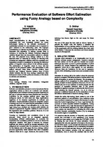
Fig. 1. Generic Software Process Model.

II. Setting the context Software performance aims at integrating performance analysis in the software domain. Historically the approach was to export performance modeling and measurements from the hardware domain to software systems. This was rather straightforward when considering the operating system domain but it assumed a new dimension when the focus was directed on applicative software. Moreover, with the increase of software complexity it was recognized that software performance could not be faced locally at the code level by using optimization techniques since performance problems often result from early design choices. This awareness pushed the need to anticipate performance analysis at earlier stages in software development [S90], [LZGS84]. In this context, several approaches have been proposed. In the following we focus on the integration of performance analysis at the earliest stages of the software life-cycle, namely software architecture and software specification. We will review the most important approaches in the general perspective of how each one integrates in the software life-cycle. Notice that we do not address performance analysis based on static analysis and metrics. To this respect other approaches have been proposed in literature whose discussion is out of the scope of the present work, e.g. [BCK98], [BM99]. To carry out our review we consider a generic model of software lifecycle as presented in Figure 1. We identify the most relevant phases in the software lifecycle. Since the approaches we are reviewing aim at addressing performance issues earlier in the software development cycle, our model is detailed with respect to the requirement and architectural phases.

January 8, 2003

DRAFT

TECHNICAL REPORT

5

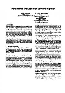
Moreover since performance is a system run time attribute we will focus on dynamic aspects of the software models used in the different phases. The various approaches differ with respect to several dimensions. In particular we consider the software dynamics model, the performance model, the phase of the software development in which the analysis is carried out, the level of detail of the pieces of information needed for the analysis, and the software architectures of the system under analysis, e.g., specific architectural pattern such as client-server, and others. All these dimensions are synthesized through the three following indicators: the integration level of the software model with the performance model, the level of integration of performance analysis in the software lifecycle and the methodology automation degree, as shown in Figure 2. We use them to classify the methodologies as reported in Section VI. The level of integration of the software and the performance models ranges from syntactically related models, to semantically related models till a unified model. This integration level qualifies the mapping that the methodologies define to relate the software design artifacts with the performance model. A high level of integration means that the performance model has a strong semantic correspondence with the software model. With the level of integration of performance analysis in the software lifecycle we identify the precise phase at which the analysis can be carried out. For each methodology we single out the software development phases in which the pieces of information required to perform the analysis has to be collected, received or supplied. The last dimension refers to the degree of automation that the various approaches can support. Figure 2 is inspired to Enslow’s model of distribution [E78]. The ideal methodology falls at the bottom of the two rightmost columns, since it should have high integration of the software model with the performance model, high level of integration with the life-cycle, that is from the very beginning, and high degree of automation. A. An example across modeling notation: the XMLTranslator System In this section we present the simple software system used throughout the paper to show different notations to model system dynamics and various performance models as described in Section III and IV, respectively. January 8, 2003

DRAFT

TECHNICAL REPORT

6

Verification & Validation Software Implementation Software Design

Integration level of the software model with the performance model.

Integration level of performance analysis in the software lifecycle Automation degree

Software Specification

Same models

Automation degree

Software Architecture Requirements

Semantically related models Syntactically related models

Automation degree Automation

deegre Low automation

Medium Automation

High Automation

Fig. 2. Classification Dimensions of Software Performance Approaches.

The software system we consider is an XMLTranslator that allows building a XML document from a text document by using a particular XML schema [XML]. The text document has a fixed structure to allow automatic identification of parts that can then be emphasized by using XML tags defined in the given Schema. The system reads a text document and creates a new XML file suitably formatted with respect to the considered XML syntax and schema. The system builds the new file by iterative steps in which it identifies useful information in the text and marks it up by the tags. Many users can concurrently request the system services, but each user cannot do multiple requests. From the description of the system we identify two software components: •

a structure builder, that preprocesses the text file to make its XML related content (i.e.,

XML special characters) conform to the XML syntax rules. The output of this step is a new syntactically different text file that is semantically equivalent to the former. This component also creates a XML file containing only the structure of the document with respect to the schema. •

a marker-up that, by using a heuristic approach, localizes useful information in the text

document, singles it out by tags of the XML schema and inserts this chunk of information in the XML file. This component works iteratively for an undefined number of times until the XML version of the document is not acceptable (i.e., it does emphasize most of the useful information under certain heuristic conditions). January 8, 2003

DRAFT

TECHNICAL REPORT

7

Structure Builder *

Marker-up

*

User User

Fig. 3. Static Software Architecture of the XMLTranslator.

The two components interact asynchronously with the structure builder component that provides input to the marker-up one. Both components can satisfy a service request at each time. We implicitly assume that input to the whole system, and therefore to the structure builder component is provided by external users. A static description of the system architecture is shown in Figure 3. In order to describe the dynamic aspects of the above system we may use one of the notation introduced in the following section. III. Software Dynamics Specification Models Software engineers describe static and dynamic aspects of a software system by using ad-hoc models. The static description consists of the identification of software modules or components and of their interconnections, e.g., 3. The dynamics of a software system concerns its behavior at run time. There exists many notations to describe the behavior of a software system. In the following we shortly review Automata, Process Algebra, Petri Nets, Message Sequence Charts (MSC), Unified Modeling Language (UML) Diagrams and Use Case Maps (UCM). A. Automata Automaton is a simple mathematical and expressive formalism that allows to model cooperation and synchronization between subsystems, concurrent and not. It is a compositional formalism where a system is modelled as a set of states and its behavior is described by transitions between them, triggered by some input symbol. More formally an automaton is composed of a (possibly infinite) set of states Q, a set of input symbols Σ and a function δ : Q × Σ → Q that defines the transitions between states. In Q there is a special state q0 ∈ Q, the initial state from which all computations start, and a set of final states F ⊂ Q reached by the system at the end of correct finite January 8, 2003

DRAFT

TECHNICAL REPORT

8

computations [HU79]. Automata can also be composed through composition operators, notably the parallel one that composes two automata A and B by allowing the interleaving combination of A and B transitions. The current state of the automaton depends on the input the system received and determines the future behavior of the system based on the next input. It is always possible to associate a direct labelled graph to an automaton, called State Transition Graph, where nodes represent the states and labelled edges represent transitions of the automata triggered by the input symbols associated to the edges. There exist many types of automata, among which we consider: deterministic automata with a deterministic transition function, that is the transition between states is fully determined by the current state and the input symbol; non deterministic automata with a transition function that allows more state transitions for the same input symbol; stochastic automata which are non deterministic automata where the next state of the system is determined by a probabilistic value associated to each possibility. A.1 XMLTralslator Automaton The state transition graph of the XMLTranslator automaton is shown in Figure 4. States are pairs of elements, that model the Structure Builder component state and the the Marker-up component state respectively. The initial state of the automaton is < q0 , q00 > where both components are inactive. This state is also the final one where the system correctly terminates the computation. Since the XMLTranslator automaton is obtained by the parallel composition of the Structure Builder and of the Marker-up components automata, we analyze their behavior separately. The Structure Builder component transits from the state q0 to the state q1 when it receives a markup request, then it starts the preprocessing phase moving to state q2 . At the end of its elaboration it sends the event markup to the Marker-up component and returns to the initial state q0 where it waits for new requests. When the Marker-up component receives the markup event, it moves from its initial state q00 to state q10 where it remains until the refinement processing has been completed. Eventually the component moves back to its initial state.

January 8, 2003

DRAFT

TECHNICAL REPORT

9

q0q 0'

Markup request

End services q0q1' refinement

q1q0' p mark u Markup request

Preprocessing

q 2q 0'

End markup q1q1'

Preprocessing

refinement

End markup q2q1'

refinement

End Preprocessing

Fig. 4. State Transition Graph for the XMLTranslator Automaton.

B. Process Algebra Process Algebras [AB84] (such as CCS [M89], CSP [H85]) are a widely known modeling technique for the functional analysis of concurrent systems. These are described as collections of entities, or processes, executing atomic actions, which are used to describe concurrent behaviors which synchronize in order to communicate. Processes can be composed by means of a set of operators, which include different forms of parallel composition. Process algebras provide a formal model of concurrent systems, which is abstract (the internal behavior of the system components can be disregarded) and compositional (systems can be modelled in terms of the interactions of their subsystems). They provide formal techniques for the verification of system properties, such as equivalences and pre-orders. Process Algebras can describe systems at different levels of abstraction. Many notions of equivalence or pre-order are defined to study the relationship between different descriptions of the same system. Behavioral equivalences allow one to prove that two different system specifications are equivalent when ”uninteresting” details are ignored, while pre-orders are suitable for proving that a low level specification is a satisfactory implementation of a more abstract one. B.1 A Process Algebra Model for the XMLTranslator system The process algebra model for the XMLTranslator system consists of two main processes, a StructureBuilder process and a Marker-up process, that perform actions to satisfy the requests. To model the asynchrony in the system we introduce two further processes representing two queues. The first queue, Queue1, buffers the requests from the users and

January 8, 2003

DRAFT

TECHNICAL REPORT

10

specification System Behaviour (User ||| User ||| User) | [enq1,arrival] | (Queue1(0,3) | [deq2] | StructureBuilder | [enq3] | Queue2(0,3) | [deq,enq2] | Marker-up ) where process User:= work; enq1; arrival; User endproc process Queue1(n,k) := [n>0] -> (deq2; Queue1(n-1,k)) [] [n (enq1; Queue1(n+1,k)) endproc process Queue2(n,k) := [n>0] -> (deq; Queue2(n-1,k)) [] [n (enq3; Queue2(n+1,k))[] [n (enq2; Queue2(n+1,k)) endproc process StructureBuilder := deq2; preprocessing; enq3; StructureBuilder endproc process Marker-up := deq; markup; ((refinement; enq2; Marker-up) [] (backtousers; arrival; Marker-up)) endproc endspec

Fig. 5. Process Algebra Model for the XMLTranslator.

generates text formatting requests for the StructureBuilder. The second queue, Queue2, models the asynchronous connection point from the StructureBuilder to the Marker-up component. The specification we present also defines a User process that models the user behavior. A user does some work, then enqueues a service request in Queue1 and waits for the results from the XMLTranslator. The behavior of the whole system is specified by putting in parallel all the processes. Fig. 5 shows the specification of the XMLTranslator system with three concurrent users and queues of capacity three, modelled by using the TIPP Process Algebra [HKMS00]. C. Petri Nets Petri Nets (PN) are a formal modeling technique to specify synchronization behavior of concurrent systems. A PN [R85] is defined by a set of places, a set of transitions, an input function relating places to transitions, an output function relating transition to places, and a marking function, associating to each place a nonnegative integer number. PN have a graphical representation: places are represented by circles, transitions by bars, input function by arcs directed from places to transitions, output function by arcs directed from transitions to bars, and marking by bullets, called tokens, depicted inside the corresponding places. Tokens distributed among places define the state of the net. The dynamic behavior of a PN is described by the sequence of transition firings. Firing rules define whether a transition is enabled or not. The main characteristics of PN are the following: •

causal dependencies and interdependencies among events may be represented explicitly.

January 8, 2003

DRAFT

TECHNICAL REPORT

11

P2

1

arrival 1 work 1 1 1

arrival 2 work 2 1

2

P1

..

Structure Builder 1 SB 1 1

.

1

arrival 3 work 3 1 1

1

2

2 P3

User 1

1 Preproc.

1

deq 2

2 SB 2

..

2 P5

User 2

Q1

2 deq 2

P6

1

2

1 11 Q0

P4

1

1

.

..

2 User 3

Marker-up M1

1 markup

M3

1

1 1 refinement 1

backtousers 1

2 M2

Q2

Fig. 6. Petri Net Model of the XMLTranslator.

A non-interleaving, partial order relation of concurrency is introduced for events which are independent of each other; •

systems may be represented at different levels of abstraction;

•

PN support formal verification of functional properties of systems.

C.1 A Petri Net for the XMLTranslator Figure 6 shows the initial configuration of the PN model corresponding to the XMLTranslator system. Each user is represented by a sub-net consisting of two places and two transitions, shown as a shaded area in the figure, and tokens in the places represent service requests. Similarly, the two system components are modelled by the corresponding sub-nets identified by the shaded area in the figure. Places labelled Q0 , Q1 , Q2 model the queues for asynchronous communication. Dynamically, user requests enter Q1 to access the Structure Builder. Then its output is enqueued in Q2 to access Marker-up. Eventually the processed request returns to the User. D. Message Sequence Charts Message Sequence Charts (MSC) is a language to describe the interaction among a number of independent message-passing instances (e.g. components, objects or processes) or between instances and the environment, specified by the International Telecommunication January 8, 2003

DRAFT

TECHNICAL REPORT

12

Union (ITU) in [ITU99]. MSC is a scenario language that describes the communication among instances, i.e., the messages sent, messages received, and the local events, together with the ordering between them. One MSC describes a partial behavior of a system. Additionally, it allows for expressing restrictions on transmitted data values and on the timing of events. MSC is also a graphical language which specify two-dimensional diagrams, where each instance lifetime is represented as a vertical line, while a message is represented by a horizontal or slanted arrow from the sending process to the receiving one. MSC supports complete and incomplete specifications and it can be used at different levels of abstraction. It allows to develop structured design since simple scenarios described by basic MSC can be combined to form more complete specifications by means of high-level MSC. In connection with other languages MSC are used to support methodologies for systems specification, design, simulation, testing, and documentation. D.1 MSC for the XMLTranslator Since the presented case study is very simple, given the similarity of the MSC description with UML Sequence Diagram one, we omit the case study description here and we refer to Section III-E.1. E. Unified Modeling Language Diagrams All the above discussed notations (except MSC) are formal specification languages so they have an exact semantics, but as a drawback, most of them are hard to use in ordinary software engineering practice. This is overcome by less precisely defined formalisms like the Unified Modeling Language [UML]. UML specified by the Object Management Group (OMG) is a notation to describe software at different levels of abstraction. It defines several types of diagrams that can be used to model different system views. Models are usually described in a visual language, which makes the modeling work easier. Even if their semantics is not formally defined, UML diagrams are well accepted because they are flexible, easy to maintain and to use. UML diagrams allow us to describe systems either statically or dynamically in an objectoriented style. Use case diagrams emphasize the interaction between a user and a system. January 8, 2003

DRAFT

TECHNICAL REPORT

13

Class diagrams show the logical view of the system by means of classes and their relationships. Interaction diagrams represent system objects and how they interact. UML defines two types of interaction diagrams: sequence diagrams and collaboration diagrams. Analogously to MSC, the former emphasizes the lifetime of each object and when interaction between objects occurs, the latter focuses on the layout to indicate how objects are statically connected. Moreover, sequence diagrams allow us to specify conditions on message sending, to use iteration marking (that identifies multiple sending of a message to receiver objects), and to define the type of communication (synchronous or asynchronous). State diagrams show the state space of a given computational unit, the events that cause a transition from one state to another, and the actions that result. Activity diagrams show the flow of system activities. Deployment diagrams show the configuration of runtime processing elements associating the software components with hardware platform. We do not consider other UML diagrams, since they are not used in our context. As listed above, UML provides many features to describe system behavior. The dynamics of a software system can be specified by using interaction diagrams which describe the message exchange among components, or by using state diagrams to specify the internal behavior of each software component, or by using activity diagrams to show the flow of the activities performed by all the components involved in the computation of interest or by using any combinations of the above diagrams. E.1 UML for the XMLTranslator The behavior of the XMLTranslator is described by the UML Sequence diagrams shown in Figure 7. It is worthwhile noting that this representation is extremely synthetic thanks to the different semantics associated to the graphical notation of the arrows representing the communication. For example, the full head arrow denotes asynchronous communication and the dashed arrow denotes return of control. The user requests a service to the XMLTranslator system by markuprequest method invocation. StructureBuilder component catches the request and processes it. When it has finished it calls the markup method on the Marker-up component, that, after some ref inement steps, returns the control to the user.

January 8, 2003

DRAFT

TECHNICAL REPORT

14

User:

StructureBuilder:

Marker-up:

Markup request:

Markup: Refinement*: Return:

Fig. 7. Sequence Diagram of the XMLTranslator.

F. Use Case Map Use Case Maps (UCM) is a graphical notation allowing the unification of the system use (Use Cases) and the system behavior (Scenarios and State Charts) descriptions [BC96]. UCM is a high-level design model to help humans express and reason about system’s largegrained behavior patterns. However, UCM does not aim at providing complete behavioral specifications of systems. At requirement level UCM models components as black boxes, and at high-level design refines components specifications to exploit their internal parts. UCM represents scenarios through paths scenarios. The start point of a map corresponds to the beginning of a scenario. Moving through the path, UCM represents the scenario in progress till its end. Paths may traverse components and are routes along which chains of causes and effects propagate through the system. F.1 UCM for the XMLTranslator Figure 8 shows the UCM model of the XMLTranslator. A user, that is represented as a component, triggers the path scenario by formulating a request. Then the path traverses the component that represents the XMLTranslator and eventually returns to the user where it has its end point. The two system components are contained in the XMLTranslator. The UCM model shows their responsibilities and how the path scenario traverses them. IV. Performance models and evaluation methods In this section we briefly introduce three main classes of stochastic performance models: Queueing Network (QN) models, Stochastic Timed Petri Nets (STPN) and Stochastic Process Algebras (SPA) [K75], [LZGS84], [ABC86], [K92], [T01], [HHK02].

January 8, 2003

DRAFT

TECHNICAL REPORT

15

User Mark-up Request

XML Translator Mark-up/ refinement Preprocessing

StructureBuilder

Marker-up

Fig. 8. UCM Model for the XMLTranslator.

Each type of performance model can be analyzed by analytical methods or by simulation in order to evaluate a set of performance indices such as resource utilization, throughput and customer response time. Simulation is a widely used general technique whose main drawback is the potential high development and computational cost to obtain accurate results. On the other hand, analytical methods require that the model satisfies a set of assumptions and constraints. These models are based on a set of mathematical relationships that characterize the system behavior. The analytical solution of these performance models relies on stochastic processes, usually discrete-space continuous-time homogeneous Markov chains (MC). Hence, we also present a short description of Markov processes. Performance analysis of complex systems feasible can be based on structuring or factorizing techniques in order to simplify the analysis. Several decomposition and aggregation techniques [K92], [BBBCC94], [KS76] and hierarchical modeling methodologies [B96], [CHIW98] have been defined for various classes of performance models. Having specific techniques for the hierarchical definition of performance models allows for the use of a hybrid approach to the solution of submodels: hybrid models are obtained when mixed (analytical and simulation) techniques are applied. Moreover, some authors propose also the combined use of different performance models for describing submodels of a given system [BBG88], [BBS02]. A. Markov processes A stochastic process is a family of random variables X = {X(t) : t ∈ T } where X(t) : T × Ω → E defined on a probability space Ω, an index set T (usually referred as time) January 8, 2003

DRAFT

TECHNICAL REPORT

16

with state space E. Stochastic processes can be classified according to the state space, the time parameter, and the statistical dependencies among the variables X(t). The state space can be discrete or continuous (processes with discrete state space are usually called chains), the time parameter can also be discrete or continuous, and dependencies among variables are described by the joint distribution function. Informally, a stochastic process is a Markov process if the probability that the process goes from state s(tn ) to a state s(tn+1 ) conditioned to the previous process history equals the probability conditioned only to the last state s(tn ). This implies that a process is fully characterized by these one-step probabilities. Moreover, a Markov process is homogeneous when such transition probabilities are time independent. Due to the memoryless property, the time that the process spends in each state is exponential or geometrically distributed for the continuous-time or discrete-time Markov process, respectively. Markov processes can be analyzed and under certain constraints it is possible to derive the stationary and the transient state probability. The stationary solution of the Markov process has a time computational complexity of the order of the state space E cardinality. Markov processes play a central role in the quantitative analysis of systems, since the analytical solution of the various classes of performance models relies on a stochastic process which is usually a Markov process. B. Queueing Network Queueing Network (QN) models have been widely applied as system performance models to represent and analyze resource sharing systems [K75], [LZGS84], [K92], [T01]. A QN model is a collection of interacting service centers representing system resources and a set of customers representing the users sharing the resources. Its informal representation is a direct graph whose nodes are service centers and edges represent the behavior of customers’ service requests. The popularity of QN models for system performance evaluation is due to the relative high accuracy in performance results and the efficiency in model analysis and evaluation. In this setting the class of product-form networks plays an important role, since they can January 8, 2003

DRAFT

TECHNICAL REPORT

17

be analyzed by efficient algorithms to evaluate average performance indices. Specifically, algorithms such as convolution and Mean Value Analysis have a computational complexity polynomial in the number of QN components. These algorithms, on which most approximated analytical methods are based, have been widely applied for performance modeling and analysis. Informally, the creation of a QN model can be split into three steps: definition, that include the definition of service centers, their number, class of customers and topology; parameterization, to define model parameters, e.g., arrival processes, service rate and number of customers; evaluation, to obtain a quantitative description of the modeled system, by computing a set of figures of merit or performance indices such as resource utilization, system throughput and customer response time. These indices can be local to a resource or global to the whole system. Extensions of classical QN models, namely Extended Queuing Network (EQN) models, have been introduced in order to represent several interesting features of real systems, such as synchronization and concurrency constraints, finite capacity queues, memory constraints and simultaneous resource possession. EQN can be solved by approximate solution techniques [LZGS84], [K92]. Another extension of QN models is the Layered Queuing Network (LQN) which allows the modeling of client-server communication patterns in concurrent and/or distributed software systems [RS95], [WNPM95], [FHMPRW95]. The main difference between LQN and QN models is that in LQN a server may become client (customer) of other servers while serving its own clients requests. LQN models can be solved by analytic approximation methods based on standard methods for EQN with simultaneous resource possession and Mean Value Analysis. Examples of performance evaluation tools for QN and EQN are Best-1, RESQ/IBM, QNAP2 and HIT [BMW94], and for LQN the LQNS tool [WNPM95], [FW98]. B.1 QN model for the XMLTranslator Figure 9 shows a QN consisting of three service centers corresponding to the Structure Builder, the Marker-up components and the users. We assume exponential service time distribution and FCFS queueing discipline. The QN topology represents the routes that January 8, 2003

DRAFT

TECHNICAL REPORT

18

t1 Structure Builder t2

N Users

1- p t3 Marker -up p

Fig. 9. QN Model for the XMLTranslator.

a user request follows to accomplish its task, where label p represents the probability that the Marker-up component has completed the iterative marking of the text. Service rates ti , 1 ≤ i ≤ 3 and number of customers N are the QN parameters. C. Stochastic Process Algebra Stochastic Process Algebra (SPA) are extensions of Process Algebras, described in Section III, aiming at the integration of qualitative-functional and quantitative-temporal aspects into a single specification technique [HHK02]. Temporal information is added to actions by means of continuous random variables, representing activity durations. Such information enriches the Label Transition System (LTS) semantic model, hence making it possible the evaluation of functional properties (e.g. liveness, deadlock), temporal indices (e.g. throughput, waiting times) and combined aspects (e.g. probability of timeout, duration of action sequences) of the modeled systems. The quantitative analysis of the modeled system can be performed by constructing, out of the enriched LTS, the underlying stochastic process. In particular, when action durations are represented by exponential random variables, the underlying stochastic process yields a Markov Chain. Various attempts have been made in order to avoid the Markov Chain state space explosion, which soon makes the performance analysis unfeasible. Some authors propose a syntactic characterization of process algebra terms whose underlying Markov Chain admits a product-form solution that could allow more efficient solution algorithms [HH95], [HT99], [S95]. Example of performance evaluation tools for SPA are the TIPP tool [HKMS00], Two Towers [BCS01], and PEPA Workbench [GH94]. January 8, 2003

DRAFT

TECHNICAL REPORT

19

specification System behaviour (User|||User|||User)|[enq1,arrival]|(Queue1(0,3)|[deq2]| StructureBuilder|[enq3]|Queue2(0,3)|[deq,enq2]|Marker-up) where process User := (work,t 1 ); enq1; arrival; User endproc process Queue1(n,k) := [n>0] -> (deq2; Queue1(n-1,k)) [] [n (enq1;Queue1(n+1,k)) endproc process Queue2(n,k) := [n>0] -> (deq;Queue2(n-1,k)) [] [n (enq3;Queue2(n+1,k)) [] [n (enq2;Queue2(n+1,k)) endproc endproc process StructureBuilder := deq2; (processing,t 2 ); enq3; StructureBuilder process Marker-up := deq; (((iteration,100000-p); (markup,t 3); enq2; Marker-up) [] ((backtousers,p); (markup,t 3 ); arrival; Marker-up)) endproc endspec

Fig. 10. TIPP Process Algebra Model for the XMLTranslator.

C.1 A SPA model for the XMLTranslator Figure 10 shows a SPA model defined by using TIPP process algebra. This model has been obtained from the model presented in Section III-B by adding performance related information to some actions. Therefore we have simple actions (e.g., enq1) and rated actions, whose rates can be used to express their execution times (e.g., (markup,t3 )) and their relative execution frequencies (e.g., (backtouser,p)). D. Stochastic Timed Petri Net Stochastic Timed Petri Net (STPN) are extensions of Petri nets, described in Section III. Petri nets can be used to formally verify the correctness of synchronization between various activities of concurrent systems. The underlying assumption in PN is that each activity takes zero time (i.e. once a transition is enabled, it fires instantaneously). In order to answer performance-related questions beside the pure behavioral ones, Petri nets have been extended by associating a finite time duration with transitions and/or places (the usual assumption is that only transitions are timed) [ABC86], [K92], [BBBCC94]. The firing time of a transition is the time taken by the activity represented by the transition: in the stochastic timed extension, firing times are expressed by random variables. Although such variables may have an arbitrary distribution, in practice the use of non memoryless distributions makes the analysis unfeasible whenever repetitive behavior is to be modeled, unless other restrictions are imposed (e.g. only one transition is enabled at a time) to simplify the analysis. The quantitative analysis of a STPN is based on the identification and solution of its

January 8, 2003

DRAFT

TECHNICAL REPORT

20

associated Markov Chain built on the basis of the net reachability graph. In order to avoid the state space explosion of the Markov Chain, various authors have explored the possibility of deriving a product-form solution for special classes of STPN. Non polynomial algorithms exist for product-form STPN, under further structural constraints. Beside the product-form results, many approximation techniques have been defined [BBBCC94]. A further extension of Petri Nets is the class of the so called Generalized Stochastic Petri Nets (GSPN), which are continuous time stochastic Petri Nets that allow both exponentially timed and untimed (or immediate) transitions [ABC86]. Immediate transition fires immediately after enabling and have strict priority over timed transitions. Immediate transitions are associated with a (normalized) weight, so that, in case of concurrently enabled immediate transitions the choice of the firing one is solved by a probabilistic choice. GSPN admit specific solution techniques [BBBCC94]. There are many performance evaluation tools for STPN and other extended classes: a database on (stochastic) Petri net tools can be found at [PND]. D.1 A STPN model for the XMLTranslator Figure 11 shows a STPN model for the XMLTranslator system, obtained from the PN model of Section III-C by introducing performance related information. In particular we are here considering a GSPN model. We assign a time attribute to all the transitions modeling the service of each component. Hence the timed transitions are: worki , 1 ≤ i ≤ 3, representing that the i − th user is formatting a text; P reproc, the StructureBuilder component is processing a request; markup, the Marker-up component is processing a request. All the remaining transitions are immediate. The transitions outgoing place M3 have a probability associated, in order to model the relative frequency of the ref inement and back alternatives. E. Simulation Models Besides being a solution technique for performance models, simulation can be a performance evaluation technique itself [BCNN99]. It is actually the most flexible and general analysis technique, since any specified behavior can be simulated. The main drawback of simulation is its development and execution cost. January 8, 2003

DRAFT

TECHNICAL REPORT

21

P2

1

2

arrival 1 work 1 1 1 t1

1 11 Q0

P1

..

2

P3

User 1

.

1 Preproc. t2

arrival 2 work 2 1 t1

2

Structure Builder 1 SB 1 1

1

P4

1

arrival 3 work 3 1 1 t1

1

2

2 P5

User 2

Q1 1

deq 2

2 deq 2

2 SB 2

..

1

.

P6

1

..

2 User 3

Marker-up M1

1 markup t3 2 M2

M3

1

1 1 refinement 1

1-p

backtousers 1

p

Q2

Fig. 11. STPN Model of the XMLTranslator.

Simulation of a complex system includes the following phases: •

building a simulation model (i.e., a conceptual representation of the system) using a

process oriented or an event oriented approach; •

deriving a simulation program which implements the simulation model;

•

verifying the correctness of the program with respect to the model;

•

planning the simulation experiments, e.g. length of the simulation run, number of run,

initialization; •

running the simulation program and analyzing the results via appropriate output analysis

methods based on statistical techniques. A critical issue in simulation concerns the identification of the system model at the appropriate level of abstraction. Existing simulation tools provide suitable specification languages for the definition of simulation models, and a simulation environment to conduct system performance evaluation, e.g., CSIM [CSIM], C++Sim [CPPSIM] and JavaSim [JSim]. V. Integrated methods for software performance engineering In this section we review approaches that propose a general methodology for software performance focussing on early predictive analysis. They refer to different specification languages and performance models, and consider different tools and environments for sysJanuary 8, 2003

DRAFT

TECHNICAL REPORT

22

tem performance evaluation. Beside them other proposals, in the literature, present ideas on model transformation through examples or case studies (e.g. [GM00], [H00], [KP99], [PK99], [P99]). Although interesting, these approaches are still preliminary thus we will not treat them in the following comparison. The various methodologies are grouped together and discussed on the basis of the type of the underlying performance model. We follow the same ordering used in Section IV to review performance models except for Markov processes that will be discussed at the end. In the same logical grouping, approaches are discussed chronologically. As introduced in Section II, our analysis refers to the general model of software life-cycle presented in Figure 1 and outlines the three classification dimensions shown in Figure 2. When meaningful, for each group of methodologies, we provide an instance of the picture of Figure 1 which shows in which phase of the software life-cycle what type of information for performance analysis is required. We differently label the pieces of information according to the various methodologies. A. Queueing Network based methodologies In this section we consider a set of methodologies which propose transformation techniques to derive QN based models (possibly EQN or LQN) from Software Architecture specifications. Some of the proposed methods are based on the Software Performance Engineering (SPE) methodology introduced by Smith in her pioneer work [S90]. A.1 Methodologies based on the SPE approach The SPE methodology [S90], [WS02], [SW02] has been the first comprehensive approach to the integration of performance analysis into the software development process, from the earliest stages to the end. It uses two models: the software execution model and the system execution model. The former takes the form of Execution Graphs (EG) that represent the software execution behavior; the latter is based on QN models and represents the system platform, including hardware and software components. The analysis of the software model gives information on the resource requirements of the software system. The obtained results, together with information about the hardware devices, are the input parameters of the system execution model, which represents the model of the whole software/hardware system. January 8, 2003

DRAFT

TECHNICAL REPORT

23

Performance Requirement Feasibility Study

Requirement Analysis

Uses of the system (use case diagram)+ Operational Profile Requirement Specification

Architectural Design Execution Environment + Scenarios + Probability (or frequency) of each scenario

Requirement Validation Service rates of Software service routines + possibly Abstract resource contention delay * Specification

Interface & Component Design

Class Diagram + Process view * + Deployment Diagram



Resource usage estimation + loops repetitions + Occurrence time of interaction ** + Hardware configuration

Fig. 12. SPE Based Approaches and the Software Process.

. The first approach based on the SPE methodology has been proposed by Williams and Smith in [WS98]. They apply the SPE methodology to evaluate the performance characteristics of a Software Architecture (SA) specified by using UML diagrams (Class and Deployment diagrams) and Message Sequence Charts extended by using UML notations. The emphasis is in the construction and analysis of the software execution model, which is considered the target model of the specified SA and is obtained from the Message Sequence Charts. The Class and Deployment diagrams contribute to complete the description of the SA, but are not involved in the transformation process. This approach was initially proposed in [SW97], which describes a case study and makes use of the tool SPE•ED for performance evaluation. In [WS02] the approach is embedded into a general method called PASA (Performance Assessment of Software Architectures) which aims at giving guidelines and methods to determine whether a SA can meet the required performance objectives. Figure 12 shows all the required information needed to carry on the described performance analysis in correspondence of the associated software process phase. For this approach such information has either a star or does not have label. SPE•ED is a performance modeling tool designed to support the SPE methodology. Users identify the key scenarios, describe their processing steps by means of EG, and specify the number of software resource requests for each step. A performance specialist provides overhead specifications, namely the computer service requirements (e.g., CPU, I/O) for the software resource requests. SPE•ED automatically combines the software models and generates a QN model, which can be solved by using a combination of analytical and

January 8, 2003

DRAFT

TECHNICAL REPORT

24

simulation model solutions. SPE•ED evaluates end-to-end response time elapsed time for each processing step, device utilization and the time spent at each computer device for each processing step. . An extension of the previous has been developed by Cortellessa and Mirandola in [CM00]. The proposed methodology called PRIMA-UML makes use of information from different UML diagrams to incrementally generate a performance model representing the specified system. This model generation technique was initially proposed in [CIM00]. The technique considered OMT-based object-oriented specification of systems (Class diagrams, Interaction diagrams and State Transition diagrams) and defines an intermediate model, called Actor-Event Graph, between the specification and the performance model. In PRIMA-UML, SA are specified by using Deployment, Sequence, and Use Case diagrams. The software execution model is derived from the Use Case and Sequence diagrams, and the system execution model from the Deployment diagram. Moreover, the Deployment diagram allows the tailoring of the software model with respect to information concerning the overhead delay due to the communication between software components. Both Use Case and Deployment diagrams are enriched with performance annotations concerning workload distribution and parameters of devices, respectively. The information required by PRIMA-UML, in the various phases of the software process, is shown in Figure 12 with no labels and double stars. In [GM02] the PRIMA-UML methodology has been extended in order to cope with the case of mobile SA by enhancing its UML description to model the mobility-based paradigms. The approach generates the corresponding software and system execution models allowing the designer to evaluate the convenience of introducing logical mobility with respect to communication and computation costs. The authors define extensions of EG and EQN to model the uncertainty about the possible adoption of code mobility. . In [CDI01] Cortellessa et alt. focus on the derivation of a LQN model from a SA specified by means of a Class diagram and a set of Sequence diagrams, generated by using standard CASE tools. The paper clearly identifies all the supplementary information needed by the method to carry on the LQN derivation. These include platform data, e.g., configuration, resource capacity, and the operational profile which includes the user

January 8, 2003

DRAFT

TECHNICAL REPORT

25

workload data. Moreover, in case of distributed software, other input documents are the software module architecture, the client/server structure, and the module-platform mapping. The method generates intermediate models to produce a global precedence graph which identifies the execution flow and the interconnections among system components. This graph, together with the workload data, the software module architecture and the client/server structure, are used to derive the extended EG. The target LQN model is generated from the extended EG and the resource capacity data. Other approaches that address the integration with Case tools will be discussed later on in this section. Other SPE-based approaches have been proposed by Petriu et alt., since they are also based on patterns we describe them in the next subsection. A.2 Architectural pattern based methodologies The approaches described hereafter consider specific classes of systems, identified by architectural patterns in order to derive their corresponding performance models. Architectural patterns characterize frequently used architectural solutions. Each pattern is described by its structure (what are the components) and its behavior (how they interact). . In [PW99], [PS02], [GP02] Petriu et alt. propose three conceptually similar approaches where SA are described by means of architectural patterns (such as pipe and filters, client/server, broker, layers, critical section and master-slave) whose structure is specified by UML Collaboration diagrams and whose behavior is described by Sequence or Activity diagrams. The three approaches follow the SPE methodology and propose systematic methods to build LQN models of complex SA based on combinations of the considered patterns. Such model transformation methods are based on graph transformation techniques. We discuss now the details of the various approaches. • In [PW99] SA are specified by using UML Collaboration, Sequence, Deployment and Use Case diagrams. Sequence diagrams are used to obtain the software execution model represented as a UML Activity diagram. The UML Collaboration diagrams are used to obtain the system execution model, that is a LQN model. Use Case diagrams provide inJanuary 8, 2003

DRAFT

TECHNICAL REPORT

26

formation on the workloads and Deployment diagrams allow for the allocation of software components to hardware sites. The approach generates the software and system execution models by applying graph transformation techniques, automatically performed by a general-purpose graph rewriting tool. • In [PS02] the authors extend the previous work by using the UML performance profile [UMLProfile] to add performance annotations to the input models, and by accepting in input UML models expressed in XML notation. Moreover the general-purpose graph rewriting tool for the automatic construction of the LQN model, has been substituted by an ad-hoc graph transformation implemented in Java. • The third approach proposed in [GP02] uses the eXtensible Stylesheet Language: Transformations (XSLT), to carry on the graph transformation step. XSLT is a language for transforming a source document expressed in a tree format (which usually represents the information in a XML file) into a target document expressed in a tree format. The input contains UML models in XML format, according to the standard XML Metadata Interchange (XMI), and the output is a tree representing the corresponding LQN model. The resulting LQN model can be in turn analyzed by existing LQN solvers after an appropriate translation in textual format. In Figure 13 all the information needed in Petriu’s approaches for performance analysis is indicated with no marks or a star. . Menascé and Gomaa presented in [MG98], [MG00] an approach to the design and performance analysis of client/server systems. It is based on CLISSPE (CLIent/Server Software Performance Evaluation), a language for the software performance engineering of client/server applications [M97]. A CLISSPE specification is composed of a declaration section containing clients and client types, servers and server types, database tables and other similar information, a mapping section allocating clients and servers to networks, assigning transactions to clients, etc., and a transaction specification section describing the system behavior. The CLISSPE system provides a compiler to generate the QN model, estimates some model parameters, and provides a performance model solver. For the specification of a client/server system the methodology uses UML Use Case diagrams to specify the func-

January 8, 2003

DRAFT

TECHNICAL REPORT

27 Performance Requirement Feasibility Study

Uses of the system + Operational profile



Architectural Design Architectural pattern + Collaboration Diagram+ Scenarios (Sequence and/ or Activity diagrams *) + Workload +Software/hardware mapping (e.g. by Deployment Diagram)+ relational DB definition **



Workload (number of loop repetitions, resource usage) *+ Hardware configuration Data Structure & Algorithm Design Implementation & Integration


Fig. 13. Architectural Pattern Based Approaches and the Software Process.

tional requirements, Class diagrams for the structural model and Collaboration diagrams for the behavioral model. From these diagrams the methodology derives a CLISSPE specification. A relational database is automatically derived from the Class diagram. The CLISSPE transaction specification section is derived (not yet automatically) from Use Case diagrams and collaboration diagrams, and references the relational database derived from the structural model. Moreover, the CLISSPE system uses information on the database accesses (of the transaction specification section) to automatically compute service demands and estimate CPU and I/O costs. In order to complete the CLISSPE declaration and mapping sections, the methodology requires the specification of the client/server architecture with the related software/hardware mapping annotated with the performance characteristics such as processor speeds, router latencies, etc. The information required by the approach in the various phases of the software process, is indicated with no marks and double stars in Figure 13. A.3 Methodologies based on trace-analysis In this subsection we consider approaches based on the generation and analysis of traces (sequence of events/actions) from dynamic description of the software system. . The first approach we consider proposes an algorithm that automatically generates QN models from software architecture specifications described by means of Message Sequence Charts (MSC)[AABI00] or by means of Labelled Transition Systems (LTS) [ABI01]. A key point of this approach is the assumption that the SA dynamics, described by MSC or LTS, is the only available system knowledge. This allows the methodology to be applied January 8, 2003

DRAFT

TECHNICAL REPORT

28

Feasibility Study



Architectural Design MSC *+ Implementation Scenario Alternatives * Scenarios + test cases + State Machines



Environment + Configuration +Workload + resource demand



Fig. 14. Trace-analysis Approaches and the Software Process.

in situations where information concerning the system implementation or deployment are not yet available. The approach analyzes the SA dynamic specification in terms of the execution traces (sequences of events) it defines, in order to single out the real degree of parallelism among components and their dynamic dependencies. Only the subsystems that actually can behave concurrently will correspond to components of the QN model corresponding to the SA description. The dynamic activation of software components and connectors is modeled by customers’ service time in the QNM. Concurrent component activation in SA is represented by customers’ concurrent activity in the QNM that possibly compete for the use of shared resources. Synchronous communication of concurrent components can be modeled by service centers with finite capacity queues and an appropriate blocking protocol, as in QNM with BAS blocking. The analysis of the QNM of the SA leads to the evaluation of some performance indices that have to be interpreted according to the model abstraction level, that is at the SA level. The model parameter instantiations correspond to potential implementation scenarios and the performance evaluation results can provide useful insights of how to carry on the development process at the SA design in terms of potential performance. Performance indices are interpreted at the SA level, by considering the meaning of the parameters instantiation. The information required by the approach is indicated with a star in Figure 14. . Woodside et. alt. describe in [WHSB01] a methodology to automatically derive a LQN model from a commercial software design environment called ObjecTime Developer [OTD98] by means of an intermediate prototype tool called PAMB (Performance Analysis Model Builder). The application domain of the methodology is real-time interactive soft-

January 8, 2003

DRAFT

TECHNICAL REPORT

29

ware and it encompasses the whole development cycle, from the design stage to the final product. ObjecTime Developer allows the designer to describe a set of communicating actor processes, each controlled by a state machine, plus data objects and protocols for communications. It is possible to “execute” the design over a scenario by inserting events, stepping through the state machines, and executing the defined actions. Moreover, the tool can generate code from the system design. The approach in [WHSB01] takes advantage of such code generating and executing scenarios capabilities for model-building. The prototype tool PAMB, integrated with ObjecTime Developer, keeps track of the execution traces, and captures the resource demands obtained by executing the generated code in different execution platforms. Essentially, the trace analysis allows the building of the various LQN submodels (one for each scenario) which are then merged into a global model, while the resource demands data provides the model parameters. After solving the model through an associated model solver, the PAMB environment reports the performance results by means of performance annotated MSC and graphs of predictions. . A more recent approach of Woodside et alt. to performance analysis from requirements to architectural phases of the software life-cycle is presented in [PW02]. This approach derives LQN performance models from system scenarios described by means of UCM. The UCM specification is enriched with performance annotation. The approach defines where and how the diagrams have to be annotated and the default values to be used when performance data are missing. The derivation of LQN models from annotated UCM is quite direct, due to the close correspondence between UCM and LQN basic elements. The derivation is defined on a path by path basis, starting from UCM start points. The identification of the component interaction types, however, is quite complex since the UCM notation does not allow the specification of synchronous, asynchronous and forwarding communication mechanisms. The approach describe an algorithm for deriving such information from the UCM paths, by maintaining the unresolved message history while traversing a UCM path. The UCM2LQN tool automatize the methodology and it has has been integrated into a general framework called UCM Navigator that allows the creation and editing of UCM,

January 8, 2003

DRAFT

TECHNICAL REPORT

30

supports scenario definitions, generates LQN models, and exports UCM as XML files. The information required by Woodside and alt.’s approaches is indicated with no label and a star in Figure 13. A.4 UML for Performance In this subsection we consider efforts that have been pursued entirely in the UML framework in order to make performance analysis possible by starting from UML software descriptions. . In [UMLProfile] the UML Profile for Scheduling, Performance and Time has been specified. It has been adopted as an official OMG standard in March 2002. In general, a UML profile defines a domain-specific interpretation of UML, it might be viewed as a package of specializations of general UML concepts that capture domain-specific variations and usage patterns. Additional semantic constraints introduced by the UML profile must conform to the standard UML semantics. To specify a profile UML extensibility mechanisms (i.e. stereotypes, tagged values, constraints) are used. Main aims of the UML Profile for Scheduling, Performance and Time (Real-time UML standard) are to identify the requirements for enabling performance and scheduling analysis of UML models. It defines standard methods to model physical time, timing specifications, timing services and logical and physical resources, concurrency and scheduling, software and hardware infrastructure and their mapping. Hence,it provides the ability to specify quantitative information directly in UML models allowing quantitative analysis and predictive modeling. This profile has been defined to facilitate the use of analysis methods and to automate the generation of analysis models and of the analysis process itself. Analysis methods considered in the profile are scheduling analysis and performance analysis based on queueing theory. . The approach introduced by Kähkipuro in [K01] is quite different from the other ones described in this section. The proposed framework consists of three different performance model representations and of the mappings among them. The starting representation is based on UML. The key point of this approach is the use of UML as a new way to represent performance models. This approach proposes a UML-based performance modeling notation (i.e., a notation compatible with the UML design description) which can be used January 8, 2003

DRAFT

TECHNICAL REPORT

31

Feasibility Study



Architectural Design Classes to represent software components and resources + Running configuration by means of UML Deployment Diagrams


Abstract Specification

One UML Collaboration or Sequence Diagrams for each workload + (Estimated) Service demand per each method of a class

Interface & Component Design

Data Structure & Algorithm Design

Scheduling policy for each resource (queue or delay) derived from communication types

Implementation & Integration


Fig. 15. Kähkipuro’s Approach and the Software Process.

in the UML specification of a system, in order to specify performance elements besides the pure functional ones. Then the UML representation is automatically mapped into a textual representation, which retains only the performance aspects of the system, and it is further translated into an extended QN model representing the simultaneous resource possessions, synchronous resource invocations and recursive accesses to resources. Such a model can be solved by using approximate or simulation techniques, and the results can be translated back to the textual representation and the UML diagrams, realizing in this way a feedback mechanism. The approach has been partially implemented in a prototipe tool called OAT (Object-oriented performance modeling and Analysis Tool). Note that this approach does not really propose a transformation methodology from a SA specification to a performance model, since the three steps (or representations) of the framework just give three equivalent views of the modeled system with respect to performance. In this approach a designer must have a performance skill, besides UML knowledge, to produce a correct diagram. However, the approach lifts up the transformation step to the specification level. In fact, in order to obtain a real model transformation methodology, it would be sufficient to add a further level on top of the whole framework, producing from usual functional oriented UML diagrams extended UML diagrams annotated with performance information. In Figure 15 we summarize the information required by Kähkipuro’s approach. B. Process Algebras based approaches Several stochastic extensions of PA have been proposed in order to describe and analyze both functional and performance properties of software specifications within the same framework. Among these we consider TIPP (TIme Processes and Performability evaluJanuary 8, 2003

DRAFT

TECHNICAL REPORT

32

ation) [HKMS00], EMPA (Extended Markovian Process Algebra) [BG98], [BCD00] and PEPA (Performance Evaluation Process Algebra) [H93], [GH94] which are all supported by appropriate tools (the TIPP tool, PEPA Workbench and Two Towers —for EMPA). All of them associate exponentially distributed random variables to actions, and provide the generation of a Markov chain out of the semantic model (LTS enriched with time information) of a system. Beside exponential actions, also passive and immediate actions are considered. The main differences among PEPA, EMPA and TIPP concern the definition of the rate of a joint activity which arises when two components cooperate or synchronize, and the use of immediate actions. Different choices on these basic issues induce differences on the expressive power of the resulting language. We refer to [HHK02] for an accurate discussion about this topic. The advantage of using PEPA, EMPA or TIPP for software performance is that they allow the integration of functional and non-functional aspects and provide a unique reference model for software specification and performance. However, from the performance evaluation viewpoint, the analysis usually refers to the numerical solution of the underlying Markov chain which can easily lead to numerical problems due to the state space explosion. On the software side, the software designer is required to be able to specify the software system using process algebras and to associate the appropriate performance parameters (i.e., activity rates) to actions. In order to overcome this last drawback, Pooley describes in [P99] some preliminary ideas on the derivation of SPA models from UML diagrams. The starting point is the specification of a SA by means of a combined diagram consisting of a Collaboration diagram with embedded Statecharts of all the collaborating objects. The idea is then to produce a SPA description out of each Statechart and then to combine the obtained descriptions into a unique model. Balsamo et alt. introduced in [BBS02] a SPA based Architectural Description Language (ADL) called Æmilia (an earlier version called ÆMPA can be found in [BCD00]), whose semantics is given in terms of EMPA specifications. Æmilia aims at facilitating the designer in the process algebra-based specification of a software architecture, by means of syntactic constructs for the description of architectural components and connections. Æmilia is also

January 8, 2003

DRAFT

TECHNICAL REPORT

33 Performance Requirements

Feasibility Study



Architectural Design



Software specification by using Stochastic Process Algebra/ Generalized Stochastic Petri Net + estimation of execution time for each action/timed transition



Fig. 16. SPA and SPN Based Approaches and the Software Process.

equipped with checks for the detection of possible architectural mismatches. Moreover for Æmilia specifications it has been proposed a translation into QN models to take advantage of the orthogonal strengths of the two formalisms: formal techniques for the verification of functional properties for Æmilia (SPA in general), and efficient performance analysis for QN. Figure 16 indicates the information required by SPA-based approaches. C. Petri Net based approaches Like Process Algebras, Petri nets are usually proposed as a unifying formal specification framework, allowing the analysis of both functional and non-functional properties of systems. There are a lot of stochastic Petri net frameworks (e.g., GreatSPN, HiQPN, DSPNExpress 2000, and many others which can be found in [PND]) allowing the specification and the functional/quantitative analysis of a Petri net model. Recently approaches to the integration of UML specifications and Petri nets have been proposed [KP99], [BDM02]. In [KP99] the authors present some ideas on the derivation of a GSPN from Use Cases diagrams and combined Collaboration and Statecharts diagrams. The idea is to translate the Statechart associated with each object of the Collaboration diagram into a GSPN (where states and transitions of the Statechart become places and transitions in the net, respectively), and then to combine the various nets into a unique model. In [BDM02] the authors propose a systematic translation of Statecharts and Sequence Diagrams into GSPN. The approach consists in translating the two type of diagrams in two separate labelled GSPN. January 8, 2003

DRAFT

TECHNICAL REPORT

34

The translation of a Statechart gives rise to one labelled GSPN per unit where a unit is a state with all its outgoing transitions. The resulting nets are then composed over places with equal label in order to obtain a complete model. Similarly, the translation of a Sequence diagram consists of modeling each message with a labelled GSPN subsystem and then composing such subsystems by taking into account the causal relationship between messages belonging to the same interaction, and defining the initial marking of the resulting net. The final model is obtained by building a GSPN model by means of two composing techniques. In Figure 16 we outline the information required by PN based approaches. D. Methodologies based on simulation methods We shall now consider two approaches based on simulation models. They use simulation packages in order to define a simulation model whose structure and input parameters are derived from UML diagrams. . The first approach, proposed by de Miguel et alt. in [DLHBP00], focuses on real time systems, and proposes extensions to UML diagrams to express temporal requirements and resource usage. The extension is based on the use of stereotypes, tagged values and stereotyped constraints. SA are specified using the extended UML diagrams without restrictions on the type of diagrams to be used. Such diagrams are then used as input for the automatic generation of the corresponding scheduling and simulation models via the Analysis Model Generator (AMG) and Simulation Model Generator (SMG), respectively. In particular, SMG generates OPNET models [OPNET], by first generating one submodel for each application element and then combining the obtained submodels into a unique simulation model. The approach provides a feedback mechanism: after the model has been analyzed and simulated, some results are included in the tagged values of the original UML diagrams. This is a relevant feature, which helps the SA designer in interpreting the feedback from the performance evaluation results. . The second approach, proposed by Arief and Speirs in [AS00], presents a simulation framework named Simulation Modeling Language (SimML) to automatically generate a simulation Java program (by means of the JavaSim tool [JSim]) from the UML specification of a system that realizes a process oriented simulation model. SimML allows the user to January 8, 2003

DRAFT

TECHNICAL REPORT

35

draw Class and Sequence diagrams and to specify the information needed for the automatic generation of the simulation model. The approach proposes a XML translation of the UML models, in order to store the information about the design and the simulation data in a structured way. E. A methodology based on stochastic processes All the approaches presented in this section so far consider QN, SPA, SPN or simulation based performance models. In this subsection we describe an approach which considers generalized semi-Markov processes, i.e. stochastic processes where general distributions (and not only memoryless ones) are allowed and the Markovian property is only partially fulfilled. . The approach in [LTKLW02] proposes a direct and automatic translation of system specifications given by UML State diagrams or Activity diagrams, into a corresponding discrete-event stochastic system, namely a generalized semi-Markov process. The first step of the approach consists of introducing extensions to UML State diagrams and Activity diagrams to associate events with exponentially distributed durations and deterministic delays. The enhanced UML diagrams are then mapped onto a generalized semi-Markov process by using an efficient algorithm for the state space generation. The approach has been implemented using the tool DSPNexpress 2000 (information in [PND]) which supports the quantitative analysis of discrete-event stochastic processes. DSPNexpress imports UML diagrams from some commercial UML design package, and adds the timing information by using a graphical user interface. The approach has two main drawbacks, namely, the use of non standard UML notation for the additional timing information and the possible state space explosion in the generation of the state transition graph out of the UML diagrams. VI. Comparison and classification In this section we provide a synthesis of the methodologies previously surveyed, in light of the several dimensions outlined in Section II. Table 1, summarizes all the methodologies and their characteristics. The first column reports the methodology’s name that will be used in Figure 17. The second and third columns indicate the behavioral and performance January 8, 2003

DRAFT

TECHNICAL REPORT

36

models, respectively. The former is the starting point of the considered methodology while the latter represents the target model for the analysis. The fourth and fifth columns consider potential constraints implied by the methodology. These can be related to the software system architecture or to a specific application domain. The lifecycle column indicates the first software development phase in which the methodology can be applied. The seventh, eighth and ninth columns are quality attributes that we derived from the study of the various methodologies. Information level represents the amount of information that has to be provided in order to make the methodology applicable. This encompasses information like operational profile, resources workloads, etc. Feedback indicates that a methodology has explicitly addressed the issue of providing some sort of feedback from performance analysis to the designer. This means, for example, that from a bad throughput figure, it is easy to single out which are the responsible software components. Automation degree refers to the suitability for automation of a methodology. It is worthwhile noticing that this does not indicate the current achieved automation, which is instead indicated in the last column. The tool column mentions the tool that supports the automated portion of the methodology, if any. Note that there is a dependency between the information level and the lifecycle phase. The more information is needed the more advanced software development phase is implied. This means that some methodologies, although starting from abstract software descriptions, are applicable only from the design level onward, as far as the lifecycle phase is concerned. The kind of detailed information required by each methodology can be found in the figures in Section V. Note that one could also imagine that these pieces of information do somehow exist, e.g., can be predicted by using execution scenarios. However, for classification purposes we consider the development phase in which this kind of information would naturally be available and relate the methodology to that phase. According to the discussion in Section II, in Figure 17 we classify the methodologies. In each internal small cube, label ordering has no meaning. Differently, when a label lies at the intersection of more cubes, like [CDI01], this indicates that the corresponding methodology has characteristics of both classes. Most of the methodologies fall in the slices of syntactically or semantically related models

January 8, 2003

DRAFT

TECHNICAL REPORT

January 8, 2003

37

DRAFT

TECHNICAL REPORT

38 Integration level of the software model with the performance model. GSPN SPA

Integration level of performance analysis in the software lifecycle

Same models

Automation degree

CDI01

WS98 LTKLW02 CM00 DHLBP00 WHSB01 GM02

MG00

AABI00

Semantically related models

Automation degree

Verification & Validation Software Implementation

AS00

Software Design

PW99 K01 PS02 GP02

Software Specification Software Architecture Automation degree

Requirements Low automation

Medium Automation

PW99 GP02 PS02 PW02

Syntactically related models Automation deegre

High Automation

Fig. 17. Classification of Considered Methodologies.

and in the layer referring to software design. Let us recall that the dimension concerning the integration level of software models with the performance models refers to the way the mapping between software models and performance models is carried out. In the slice of syntactically related models we put the methodologies that integrate the design and the performance models based on structural-syntactical mappings. These means that the analysis of the dynamic behavior of the design model does not play a driving role in the mapping. For example in [PW02] there is an explicit correspondence between syntactic elements at the design level and elements of the performance model, e.g., UCM components and LQN tasks. The slice of semantically related models refers to methodologies whose mapping between design and performance models is mainly based on the analysis of the dynamic behavior of the design artifacts. For example, in [WHSB01] the mapping is based on the analysis of the state machines model of the system design. The last slice singles out the methodologies that allow the use of the same model both for design description and performance analysis. This slice can actually be seen as a particular

January 8, 2003

DRAFT

TECHNICAL REPORT

39 Rational Rose

...

ArgoUML

SPEED PAMB

Software Specification

UCM2LQN

... UCM Navigator

Performance Model Generation

HiQPN-Tool GreatSPN

TIPPtool

Performance Model Evaluation

PEPA Workbench TwoTowers

DSPNexpress 2000 SimML AMG

CSim

ResQ HiQPN-Tool

...

Fig. 18. Tools and Performance Process.

case of the semantically related models one when the mapping is the identity modulo timing information. However, we decide to keep it separate because this ideal integration can be obtained only if the software designer has the skill to work with sophisticated specification tools. Figure 18 shows the three stages of any software performance analysis process and of the automation tools that can apply in these stages. Arrows indicate that the corresponding tools support the automation of a stage or of the set of stages enclosed in the box the arrow points to. The dashed arrow going from performance model evaluation to software specification represents the analysis of potential feedback. It is dashed since, so far, not all the tools pointing to the largest box automatically support this feature. The picture shows that most of the tools apply to the whole process providing a comprehensive environment. On the other hand several tools, with different characteristics, exist that automate single stages of the process. This suggests to investigate the possibility to provide an integration framework where the tools automating single stages of the process can be plugged in to provide a user with a best-fit analysis framework. VII. Conclusions In this paper we have presented the state of the art in software performance. We have taken a software-designer perspective in order to classify and evaluate the growing number of approaches presented in the last years. Our choice is driven by the generally acknowledged awareness that the lack of performance requirement validation in current January 8, 2003

DRAFT

TECHNICAL REPORT

40

software practice is mostly due to the knowledge gap between software engineers/architects and quality assurance experts rather than to foundational issues. Moreover, short time to market requirements make this situation even more critical. In this scenario expressive and intuitive notations, coupled with automated tools for performance validation, would allow quantitative numerical results to be interpreted as design feedback, thus supporting quick and meaningful design decisions. This is confirmed by the classification we carried out. Referring to Figure 17 it clearly appears that almost all methodologies try to encompass the whole software life-cycle starting from early software artifacts. It is also meaningful that most methodologies are tightly coupled with tool support that allows the automation of (portion of) them. Like there is no methodology which is fully supported, there is no methodology that does not provide or foresees automation. Most approaches try to apply performance analysis very early, typically at the software architecture level. So far, most of them still require many pieces of detailed information on the implementation/execution scenarios in order to carry on performance analysis. Nevertheless there is a growing number of attempts that try to relax implementation/execution constraints to make the analysis applicable at abstract design levels. Three indications clearly come out of this survey. The first is about software design specifications, the second is about performance models and the third one is related to the analysis process. For software design specifications we believe that the trend is in using standard practice software artifacts, like UML diagrams. Queuing Networks and their extensions candidate as performance models. QN provide an abstract/black-box notation, thus allowing easier feedback and model comprehension, especially in a component-based software development. As far as the analysis process is concerned, feedback besides the actual performance analysis is a key success factor for a widespread use of this kind of methodologies. Obviously, several problems still remain to be studied and solved. Software notations should allow for easily expressing performance related attributes and requirements. The more abstract software notation is used the more difficult the mapping to the performance model is. For QN this is a problem that can only be amended by the existence of algorithms

January 8, 2003

DRAFT

TECHNICAL REPORT

41

and tools that permit the creation of performance models from standard software artifacts. This is not a problem for GSPN and SPA provided that the designers use these same notations for the behavioral descriptions, which, in software practice, is rarely the case. Therefore, if we assume a standard development process, with standard software artifacts, like UML-based ones, the effort to produce the performance model from the behavioral description is comparable for all three models. Another problem concerns the complexity of the obtained performance model. This sometimes might prevent efficient model evaluation. The existence of a strong semantic mapping between the software artifacts and the performance model may suggest strategies to reduce the performance model complexity still maintaining a meaningful semantic correspondence. Complexity problems can also be addressed by using simulation techniques besides analytical ones. Last but not least the whole analysis process asks for automatic support. How to provide useful feedback is an important issue that deserves more study and experiments. Summarizing, we believe that from this survey it emerges that although no comprehensive methodology is at present available, the field of software performance is mature enough for approaches that can be profitably put in practice. References [AABI00]

F. Andolfi, F. Aquilani, S. Balsamo, P. Inverardi, ”Deriving Performance Models of Software Architectures from Message Sequence Charts”, In [WOSP00], pp. 47–57, 2000.

[AB84]

D.Austry, G. Boudol, ”Algébre de processus et synchronization”. Theoretical Computer Science, Vol. 30, No.1, pp. 91–131, 1984.

[ABC86]

M. Ajmone, G. Balbo, G. Conte, ”Performance Models of Multiprocessor Performance”, The MIT Press, 1986.

[ABI01]

F. Aquilani, S. Balsamo, P. Inverardi, ”Performance Analysis at the software architecture design level”, Performance Evaluation, Vol. 45, No.4, pp. 205–221, 2001.

[AS00]

L.B. Arief, N.A. Speirs, ”A UML Tool for an Automatic Generation of Simulation Programs”, In [WOSP00], pp. 71–76, 2000.

[B96]

P. Buchholz, ”A framework for the hierarchical analysis of discrete event dynamic systems”, Phd Thesis, University of Dortmund, 1996.

[BBBCC94]

F. Baccelli, G. Balbo, R.J. Boucherie, J. Campos, G. Chiola, ”Annotated bibliography on stochastic Petri nets”. In Performance Evaluation of Parallel and Distributed Systems — Solution Methods, CWI Tract, 105, pp. 1–24, Amsterdam, 1994.

[BBG88]

January 8, 2003

G. Balbo, S. Bruell, S. Ghanta, ”Combining queueing networks and generalized stochastic Petri

DRAFT

TECHNICAL REPORT

42

nets for the solution of complex models of system behaviour”, IEEE Transactions on Computers, Vol. 37, pp. 1251–1268, 1988. [BBS02]

S. Balsamo, M. Bernardo, M. Simeoni, ”Combining Stochastic Process Algebras and Queueing Networks for Software Architecture Analysis”. In [WOSP02], pp. 190–202, 2002.

[BC96]

R.J.A. Buhr, R.S.Casselman, ”Use CASE Maps for Object-Oriented Systems” Prentice Hall, 1996.

[BCD00]

M. Bernardo, P. Ciancarini, L. Donatiello, ”ÆMPA: A Process Algebraic Description Language for the Performance Analysis of Software Architectures” In [WOSP00], pp. 1–11, 2000.

[BCK98]

L. Bass, P. Clements, R. Kazman, ”Software Architecture in Practice”. SEI Series in Software Engineering, Addison-Wesley, 1998.

[BCNN99]

J. Banks, J. S. Carson II, B. L. Nelson, D. M. Nicol, ”Discrete-event System Simulation”, Prentice

[BCS01]

M.

Hall, 1999. Bernardo,

W.R.

Cleaveland,

W.S.

Stewart,

”TwoTowers

1.0

User

Manual”,

http://www.sti.uniurb.it/bernardo/twotowers/ , 2001. [BDM02]

S. Bernardi, S. Donatelli, J. Meseguer, ”From UML Sequence Diagrams and Statecharts to analysable Petri Net models”, In [WOSP02], pp. 35–45, 2002.

[BG98]

M. Bernardo, R. Gorrieri, ”A Tutorial on EMPA: A Theory of Concurrent Processes with Nondeterminism, Priorities, Probabilities and Time”, Theoretical Computer Science, Vol. 202, pp. 1–54, 1998.

[BM99]

Jan Bosh, Peter Molin, ”Software Architecture Design: Evaluation and Transformation”, Proceedings of the 1999 IEEE Engineering of Computer Systems Symposium, pp. 4–10, December 1999.

[BMW94]

H. Beilner, J. M¨ ater, C. Wysocki, ”The hierarchical evaluation tool HIT”, Proceedings of the 7th International Conference on Modelling Techniques and Tools for Computer Performance Evaluation, Wien, 1994.

[CDI01]

V. Cortellessa, A. D’Ambrogio, G. Iazeolla, ”Automatic derivation of software performance models from CASE documents”, Performance Evaluation, Vol. 45, pp. 81–105, 2001.

[CHIW98]

P.S. Coe, F.W. Howell, R.N. Ibbett, L.M. Williams, ”Technical Note: A Hierarchical Computer Architecture Design and Simulation Environment”, ACM Transactions on Modelling and Computer Simulation, Vol. 8, No. 4, pp. 431–446, 1998.

[CIM00]

V. Cortellessa, G. Iazeolla, R. Mirandola, ”Early generation of performance models for objectoriented systems”, IEE Proceedings-Software, Vol. 147, No. 3, pp. 61–72, 2000.

[CM00]

V. Cortellessa, R. Mirandola, ”Deriving a Queueing Network based Performance Model from UML Diagrams”, In [WOSP00], pp. 58–70, 2000.

[CPPSIM]

”C++Sim” - at http://cxxsim.ncl.ac.uk/

[CSIM]

”CSIM - Performance Simulator” - at http://www.atl.imco.com/proj/csim

[DLHBP00]

M. De Miguel, T. Lambolais, M. Hannouz, S. Betgé-Brezetz, S. Piekarec, ”UML Extensions for the Specification and Evaluation of Latency Constraints in Architectural Models”, In [WOSP00], pp. 83–88, 2000.

[E78]

P. H. Enslow Jr, ”What is a “distributed” data processing system?”, Computer, 11(1), pp. 13–21, January 1978.

[FHMPRW95] G. Franks, A. Hubbard, S. Majumdar, D.C. Petriu, J. Rolia, C.M. Woodside, ”A toolset for

January 8, 2003

DRAFT

TECHNICAL REPORT

43

Performance Engineering and Software Design of Client-Server Systems”. Performance Evaluation, Vol. 24, No. 1–2, pp. 117–135, 1995. [FW98]

R. Franks, C.M. Woodside, ”Performance of multi-level client-server systems with parallel service operations”, in [WOSP98], pp. 120–130, 1998.

[GH94]

S. Gilmore, J. Hillston, ”The PEPA Wokbench: A Tool to Support a Process Algebra-based Approach to Performance Modelling”, Proceedings of the 7th International Conference on Modelling Techniques and Tools for Performance Evaluation, Springer LNCS 794, pp. 353–368, 1994.

[GHR92]

N. G¨ otz, U. Herzog, M. Rettelback, ”TIPP—a language for timed processes and performance evaluation”, Technical Report 4/92, IMMD7, University of Erlangen-N¨ urnberg, Germany, 1992.

[GM00]

H. Gomaa, D.A. Menascé, ”Design and Performance Modeling of Component Interconnection Patterns for Distributed Software Architectures”, In [WOSP00], pp. 117–126, 2000.

[GM02]

V. Grassi, R. Mirandola, ”PRIMAmob-UML: A Methodology for Performance Analysis of Mobile Software Architectures”, In [WOSP02], pp. 262–274, 2002.

[GP02]

G. Gu, Dorina C. Petriu, ”XSLT transformation from UML models to LQN performance models”, In [WOSP02], pp. 227–234, 2002.

[H85]

C.A.R. Hoare, ”Communitating sequential processes”, Prentice-Hall Int., London, 1985.

[H93]

J. Hillston, ”PEPA - Performance Enhanced Process Algebra”, Technical Report CSR-24-93, Dept. of Computer Science, University of Edimburgh, 1993.

[H00]

F. Hoeben, ”Using UML Models for Performance Calculation”, In [WOSP00], pp. 77–82, 2000.

[HH95]

P.G. Harrison, J. Hillston, ”Exploiting Quasi-Reversible Structures in Markovian Process Algebra Models”, Computer Journal, Vol.38, No.7, pp. 510–520, 1995.

[HHK02]

H. Hermanns, U. Herzog, J.P. Katoen, ”Process Algebra for Performance Evaluation”, Theoretical Computer Science, Vol 274 (1–2), pp. 43–87, 2002.

[HKMS00]

U. Herzog, U. Klehmet, V. Mertsiotakis, M. Siegle, ”Compositional Performance Modelling with the TIPPtool”, Performance Evaluation, Vol. 39, No. 1–4, pp. 5–35, 2000.

[HT99]

J. Hillston, N. Thomas, ”Product Form Solution for a Class of PEPA Models”, Performance Evaluation, Vol.35, No.3, pp. 171–192, 1999.

[HU79]

J.E. Hopcroft, J.D. Ullman, ”Introduction to automata theory, languages and computations”, Addison-Wesley, 1979.

[ITU99]

ITU - Telecommunication Standardization Sector, ”Message Sequence Charts, ITU-T Recommentation Z.120(11/99)”, 1999.

[JSim]

JavaSim - at http://javasim.ncl.ac.uk/

[K75]

L. Kleinrock, ”Queueing Systems. Vol. 1: Theory”, Wiley, 1975.

[K92]

K. Kant, ”Introduction to Computer System Performance Evaluation”, McGraw-Hill, 1992.

[K01]

P. K¨ ahkipuro, ”UML-based Performance Modeling Framework for Component-Based Distributed Systems”, Proceedings of Performance Engineering, Springer LNCS 2047, pp. 167–184, 2001.

[KP99]

P. King, R. Pooley, ”Derivation of Petri Net Performance Models from UML Specifications of Communication Software”, Proceedings of XV UK Performance Engineering Workshop, 1999.

[KS76]

J.G. Kemeny, J.L. Snell, ”Finite Markov Chains”. Springer, New York, 1976.

[LTKLW02]

C. Lindemann, A. Th¨ ummler, A. Klemm, M. Lohmann, O. P. Waldhorst, ”Performance Analysis of Time-enhanced UML Diagrams Based on Stochastic Processes”, In [WOSP02], pp. 25–34, 2002.

[LZGS84]

January 8, 2003

E. D. Lazowska, J. Zahorjan, G. Scott Graham, K. C. Sevcik, ”Quantitative System Performance:

DRAFT

TECHNICAL REPORT

44

Computer System Analysis Using Queueing Network Models”, Prentice-Hall, Englewood Cliffs, 1984. [M89]

R. Milner, ”Communication and Concurrency”, Prentice-Hall International, International Series on Conputer Science, 1989.

[M97]

D. A. Menascé, ”A Framework for Software Performance Engineering of Client/Server Systems”, Proceedings of the 1997 Computer Measurement Group Conference, Orlando, Florida, 1997.

[MG98]

D. A. Menascé, H. Gomaa, ”On a Language Based Method for Software Performance Engineering of Client/Server Systems”, In [WOSP98], pp. 63–69, 1998.

[MG00]

D. A. Menascé, H. Gomaa, ”A Method for design and Performance Amodeling of Client/Server Systems”, IEEE Transacion on Software Engineering, Vol. 26, No. 11, pp. 1066–1085, 2000.

[OPNET]

OPNET Manuals, Mil 3, Inc., 1999.

[OTD98]

ObjecTime Ltd., Developer 5.1 Reference Manual, ObjecTime Ltd., Ottawa, Ont., 1998.

[P99]

R. Pooley, ”Using UML to Derive Stochastic Process Algebra Models”, Proceedings of XV UK

[PK99]

R. Pooley, P. King, ”The Unified Modeling Language and Performance Engineering”. Proceedings

Performance Engineering Workshop, pp. 23–34, 1999. of IEE Software, pp. 2–10, 1999. [PND]

Petri nets tools database http://www.daimi.aau.dk/PetriNets

[PS02]

Dorina C. Petriu, H. Shen, ”Applying UML Performance Profile: Graph Grammar-Based Derivation of LQN Models from UML Specifications”, Proceedings of the 7th International Conference on Modelling Techniques and Tools for Performance Evaluation, Springer LNCS 794, pp. 159–177, 2002.

[PW02]

Dorin C. Petriu, C.M. Woodside, ”Software Performance Models from System Scenarios in Use Case Maps”, Proceedings of TOOLS02, Springer Verlag LNCS 2324, pp. 141–1158, 2002.

[PW99]

Dorina C. Petriu, X. Wang, ”From UML descriptions of High-Level Software Architectures to LQN Performance Models”, Proceedings of AGTIVE’99, Springer Verlag LNCS 1779, pp. 47–62, 1999.

[R85]

W. Reisig, ”Petri Nets: an introduction”. EATCS Monographs on Theoretical Computer Science, vol. 4, 1985.

[RBPEL91]

J. Rambaugh, M. Blaha, W. Premerlani, F. Eddy, W. Lorensen, ”Object-Oriented Modeling and Design”, Upper Saddle River, H.J.: Prentice-Hall, 1991.

[RS95]

J.A. Rolia and K.C. Sevcik, ”The Method of Layers”, IEEE Transaction on Software Engineering, Vol. 21/8, pp. 682–688, 1995.

[S90]

C.U. Smith, ”Performance Engineering of Software Systems”, Addison Wesley, 1990.

[S95]

M. Sereno, ”Towards a Product Form Solution for Stochastic Process Algebras”, Computer Journal, Vol 38, No.7, pp. 622–632, 1995.

[SW02]

C.U. Smith, L.G. Williams, ”Performance Solutions: A Practical Guide to Creating Responsive, Scalable Software”, Reading, MA, Addison-Wesley, 2002.

[SW97]

C.U. Smith, L.G. Williams, ”Performance Engineering Evaluation of Object-Oriented Systems with SPE•EDT M ”, Springer Verlag LNCS 1245, pp. 135–153, 1997.

[T01]

K. S. Trivedi, ”Probability and Statistics with Reliability, Queuing, and Computer Science Applications”, John Wiley and Sons, 2001.

January 8, 2003

DRAFT

TECHNICAL REPORT

[WHSB01]

45

C.M. Woodside, C. Hrischuk, B. Selic, S.Brayarov, ”Automated performance modeling of software generated by a design environment”, Performance Evaluation, Vol 45, pp. 107–123, 2001.

[WNPM95]

C.M. Woodside, J. Neilson, S. Petriu, S. Mjumdar, ”The Stochastic rendezvous network model for performance of synchronous client-server-like distributed software”, IEEE Transaction on Computer, Vol. 44, pp. 20–34, 1995.

[WOSP98]

ACM Proceedings of Workshop on Software and Performance, WOSP’98, Santa Fe, New Mexico, 1998.

[WOSP00]

ACM Proceedings of Workshop on Software and Performance, WOSP2000, Ottawa, Canada, 2000.

[WOSP02]

ACM Proceedings of Workshop on Software and Performance, WOSP2002, Rome, Italy, 2002.

[WS98]

L.G. Williams, C.U. Smith, ”Performance Evaluation of Software Architectures”, In [WOSP98], pp. 164–177, 1998.

[WS02]

L.G. Williams, C.U. Smith, ”PASA: A Method for the Performance Assesment of Software Architectures”, In [WOSP02], pp. 179–189, 2002.

[UML]

”Unified

Modeling

Language

(UML),

version

1.4”.

OMG

Documentation.

At

http://www.omg.org/technology/documents/formal/uml.htm . [UMLProfile]

Object Management Group, ”UML Profile, for Schedulability, Performance, and Time”, OMG document ptc/2002-03-02 at http://www.omg.org/cgi-bin/doc?ptc/2002-03-02.

[XML]

”Extensible Markup Language (XML) 1.0 (Second Edition)”, W3C Recommendation 6 October 2000, At http://www.w3.org/TR/2000/REC-xml-20001006 .

January 8, 2003

DRAFT

Software Performance - Semantic Scholar

Software Performance - Semantic Scholar

Suggest Documents

Software Performance Engineering of Component ... - Semantic Scholar

Predicting Software Component Performance: On ... - Semantic Scholar

Performance Evaluation for Software Migration - Semantic Scholar

Performance Evaluation of Software Effort ... - Semantic Scholar

Software Performance Model-Driven Architecture - Semantic Scholar

Software Performance Engineering of Component ... - Semantic Scholar

Optimizing High Performance Software Libraries - Semantic Scholar

Performance Evaluation for Software Migration - Semantic Scholar

Performance Evaluation of Software Development ... - Semantic Scholar

Statistical Inference of Software Performance ... - Semantic Scholar

Software Performance Evaluation Utilizing UML ... - Semantic Scholar

Parametric Performance Contracts for Software ... - Semantic Scholar

Software, Performance, or Engineering? - Semantic Scholar

Software Performance AntiPatterns: Common ... - Semantic Scholar

Software Performance Models from System ... - Semantic Scholar

Software, Performance, or Engineering? - Semantic Scholar

Integrating Software and Hardware Performance ... - Semantic Scholar

Software implementation and performance ... - Semantic Scholar

Boosting the Performance of PC-based Software ... - Semantic Scholar

Three performance models at work: a software ... - Semantic Scholar

Integrating Software Performance Curves with the ... - Semantic Scholar

Uncertainty profile and software project performance - Semantic Scholar

Analysis and Performance Evaluation of Software ... - Semantic Scholar

Software performance modelling using PEPA nets - Semantic Scholar