Software Quality Prediction Models Compared - CiteSeerX

Software Quality Prediction Models Compared R¨udiger Lincke, Tobias Gutzmann and Welf L¨owe School of Computer Science, Physics and Mathematics Linnaeus University 35195 V¨axj¨o, Sweden Email: {rudiger.lincke|tobias.gutzmann|welf.lowe}@lnu.se

Abstract—Numerous empirical studies confirm that many software metrics aggregated in software quality prediction models are valid predictors for qualities of general interest like maintainability and correctness. Even these general quality models differ quite a bit, which raises the question: Do the differences matter? The goal of our study is to answer this question for a selection of quality models that have previously been published in empirical studies. We compare these quality models statistically by applying them to the same set of software systems, i.e., to altogether 328 versions of 11 open-source software systems. Finally, we draw conclusions from quality assessment using the different quality models, i.e., we calculate a quality trend and compare these conclusions statistically. We identify significant differences among the quality models. Hence, the selection of the quality model has influence on the quality assessment of software based on software metrics.

I. I NTRODUCTION Software analysis and quality assessment as supported by product metrics1 receive quite some attention by the research community. Efforts are directed to both the development of (object-oriented) product metrics [3]–[5] and on their validation [6]–[10]. The latter is particularly important since metrics are of little value by themselves unless there is empirical evidence that they are correlated with important external (quality) attributes [11]. Such a correlation allows using the metrics in the assessment and prediction of software quality, which is input to quality-control and -management, and to general planning activities. As discussed by Briand [12], Fenton [13], and Kitchenham [14], we distinguish two types of validation: theoretical and empirical validation. Theoretical validation ensures that a product metric is a proper numerical characterization of the property it claims to measure. Empirical validation demonstrates that a product metric is associated with some important quality attributes, e.g., correctness or maintainability. Theoretical validations have shown that certain program constructs have a causal relationship with some qualities [15]– [17]. The current theoretical framework for explaining the effect of the structural properties of object-oriented programs on quality attributes has been justified empirically [18]. Most studies agree that highly cohesive, sparsely coupled, and low inheritance programs are less likely to contain faults and 1 Literature

distinguishes between the notions ”metric” and ”measure” [1]. We use ”metric” to be consistent with ISO 9126 [2], which defines a ”software quality metric” as a ”quantitative scale and method which can be used to determine the value a feature takes for a specific software product.”

are easier to maintain. The empirical validation of objectoriented product metrics [18]–[20] shows evidence for the predictive validity of many product metrics. As a matter of fact, the metrics proposed in the Chidamer and Kemerer metrics suite [3] are even integrated in industrial strength software development tools like Rational Rose2 and Together3 . Existing empirical validation studies collect product metrics as independent variables and aim at predicting either software faults or maintenance costs as dependent variables by applying a variety of so-called software prediction models. A software quality prediction model, in short a quality model, maps metrics values to a quality attribute. Depending on the product, company, branch, customer, etc., different quality attributes might be interesting, but some of them are generally positive, e.g., few faults or low maintenance costs. The validations aim at predicting such positive quality attributes with the help of product metrics and quality models. For statistical validations, the quality attributes need to be assessed quantitatively as well, independently of the metrics and the quality models. Therefore, the number of software faults is derived from tests or bug databases [8]–[10], [18], [21]. The maintenance costs are more difficult to determine and usually approximated through maintenance effort. This effort is measured by means of the time spent on performing a maintenance task [6], [22], the changes performed [21], [23], [24], or the maintainability index (MI) [25]. The changes made in the code is in most cases approximated by number of lines of code changed. MI is a statistically validated quality model itself that is based on various product metrics4 . Hence it is considered trustworthy. As a consequence of the varying experimental setups of the validation studies, literature suggests quite a large number of different quality models based on different product metrics. All of them are validated to assess and predict the one or the other general notion of software quality, but they are validated using different sample data and dependent and independent variables. This makes it difficult for both researchers and practitioners to decide which quality model is trustworthy. It 2 http://www-01.ibm.com/software/awdtools/developer/rose/ 3 http://www.borland.com/us/products/together/index.html 4 MI combines several metrics including: the avg. Halstead volume per module, the avg. extended cyclomatic complexity per module, the avg. lines of code per module, and the avg. percent of lines of comments per module. However, a correlation of this metric and the actual “maintainability” has been shown in several studies [25].

is not even known if these models differ in their assessments and the resulting conclusions. This study answers these questions for a number of selected quality models. The remainder of this paper has the following structure: Section II discusses the background of our validation study. Section III summarizes the design of the experiment. Section IV discusses data collection and measurement, evaluation, and analysis. Section V concludes this paper and presents future work. The appendix provides complementary information regarding the selection of one of the investigated quality models. II. BACKGROUND Eurocontrol developed, together with its partners, a high level design of an integrated Air Traffic Management (ATM) system across all ECAC States5 . It was planned to supersede the current collection of individual national systems. The system architecture, called Overall ATM/CNS Target Architecture (OATA), is a UML specification. As external consultants, we supported the structural assessment of the architecture using a metrics-based approach using our software metrics tool VizzAnalyzer6 . The pilot validation focused only on a subsystem, consisting of 8 modules and 70 classes, of the complete architecture. We jointly defined the set of product metrics which quantify the architecture quality – a subset of the UML specification (basically class and sequence diagrams). Since no best practice existed, we defined our own software quality prediction model based on ISO 9126. We used the Factor-Criteria-Metric approach of McCall [26] but defined our own quantitative relationship between metrics, quality attributes, and quality factors, mainly based on our intuition. During this definition process, we had to choose from several equally intuitive variants and we neither had the time nor the resources to evaluate all of them. During evaluation of our assessment, Eurocontrol raised two questions which we could not answer in a satisfactory way: Q1 [validity of the quality model] Do the suggested and different alternative software quality prediction models calculate comparable results for the same input? Q2 [validity of the conclusions] If not, does this matter? More specifically, do these differences lead to different conclusions? In the following, we describe the experiment and conclusions that aim at answering these questions. We use a larger statistical basis than the OATA project could provide. III. E XPERIMENT D ESIGN A. Experiment Definition We define our experiment to analyze different software quality prediction models (Section III-C). The purpose is to find out differences in the prediction functions and in the conclusions drawn. We take the point of view of the 5 European Civil Aviation Conference; an intergovernmental organization with ore than 40 European states. 6 http://www.arisa.se

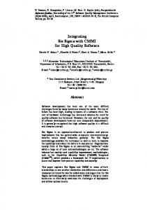
practitioner in software quality management assessing several versions of the same project. B. Planning the Experiment 1) Context Selection: The environment in which the experiment is executed is open-source Java projects. Generalization to other projects will be discussed in Section III-D as a threat to the experiment. Two of the authors of this paper conduct the experiment. The experiment addresses a problem observed in practice. 2) Hypothesis Formulation: We want to know if different software quality prediction models QM provide different assessments of software quality attributes Q0 when applying them to the same system(s). Furthermore, to compare conclusions regarding a quality trend, we assess several versions of the same test systems. The typical approach for evaluating software quality in object-oriented systems is to assess quality on class level with the help of a number of software quality metrics, and then to aggregate the different metrics values of different classes to one value on system level. First, we apply software metrics to a software system and calculate a specific metrics value for each class in the system and each metric of the quality model. Let Ci,j,k denote a class k in a version j of a software system i. Ml (Ci,j,k ) is the value for metric l of class Ci,j,k . Considering L different metrics, I software systems each in Ji different versions each in turn containing Ki,j classes, results in a huge amount of information. To reduce it, different software quality prediction models QMn aggregate some or all values Ml (Ci,j,k ) to a quality Qn (Ci,j,k ) per class Ci,j,k , and summarize Qn (Ci,j,k ) for all classes of one version to a quality Q0n (Si,j ) on system level. While we use different quality models QMn to integrate the metrics values per class Qn (Ci,j,k ), we use the same aggregation QM 0 to integrate these per class quality values to system level quality Q0n (Si,j ), see Figure 1. Secondly, we aim at drawing conclusions from the system level quality values. For our experiment, we draw conclusions based on the quality trend. In other words, we ask if for a project i the quality Q0n (Si,j ) is improving over the version j, or if it is constant or even deteriorating. Therefore, we normalize the values Q0n (Si,j ) such that 1 is the worst quality and 0 is the best quality for each of the quality models QM1..N , and aggregate the values Q0n (Si,j ) for different versions of a system to a common trend value Tn,i . Therefore, we use the slope of the linear regression function regn,i = an,i j + bn,i of each project i over its versions j. Our trend conclusion Tn,i is improving iff an,i is negative, “deteriorating” iff an,i is positive, and “constant” iff it is (close to) zero. As already discussed in the introduction, it is possible to choose from several software quality models. These define the aggregation of individual metrics to the quality Q of a class. Q is then aggregated to the quality Q0 of a system and, hence, allows to come to different trend conclusions T about the quality of the system. We formalize the resulting research questions with the following hypotheses:

€

M1 (Ci, j,k )

QM1 → Q1 (Ci, j,k ) → QM'→ Q'1 (Si, j )

M 2 (Ci, j,k )

QM 2 → Q2 (Ci, j,k ) → QM'→ Q'2 (Si, j )

 M L (Ci, j,k )

 QM N → QN (Ci, j,k ) → QM'→ Q'N (Si, j )

Fig. 1: Aggregating metrics values for classes to system level using different quality models. € Q1 Null hypothesis: There is no principle difference in the software quality Q01..N measured by the same metrics M1..L applied to the same test systems Si,j and aggregated with different quality models QM 0 • QM1..N , i.e., H0 : Q01 (Si,j ) = f2 (Q02 (Si,j )) = . . . = fN (Q0N (Si,j )) with linear functions f . Alternative hypothesis: There is no such set of linear functions f , i.e., H1 : Q01 (Si,j ) 6= f2 (Q02 (Si,j )) 6= . . . 6= fN (Q0N (Si,j )) for linear functions f . Measures needed: metrics values per class M1..L (Ci,j,k ), software quality values per class Q1..N (Ci,j,k ), and software quality values per system Q01..N (Si,j ). Q2 Null hypothesis: There is no difference in the conclusions Tn,i based on different qualities Q01..N (Si,j ) resulting from different quality models QM 0 • QM1..N for the versions j ∈ [1 . . . Ji ] of the same test project i, i.e., H0 : T1,i = . . . = TN,i Alternative hypothesis: There is a difference, i.e., H1 : T1,i 6= . . . 6= TN,i Measures needed: trend conclusions per system T1..N,i based on software quality values per system Q01..N (S1..J,j ). 3) Variable Selection: The independent variable is the quality model QM . The dependent variable is the system level software quality Q0 and resulting trend conclusions T . 4) Selection of Subjects/Objects: First, we consider variants of an ISO 9126-based quality model. Additionally, we consider quality models from literature, but we limit ourselves to evaluating only those based on similar evaluation approaches and on the same input metrics. Using models with a too diverse set of input metrics would increase the effort for collecting these metrics beyond our resources. Thus, we omit approaches involving Neural Networks etc. for integrating and aggregating the individual class level metrics values. The selected quality models are a sample of models discussed in literature, but not a random sample. Second, we limit ourselves to a single software metric tool, VizzAnalyzer, since repeating the experiment with several tools would require a much higher effort on measurement, data collection, evaluation, and analysis. In fact, we have shown earlier that different metrics tools lead to different class level quality values for the same system(s) and the same quality model and even to different conclusions regarding the quality ranking of the classes [27]. Third, the quality models and the metrics tool limit, in

turn, the selection of software quality metrics. The selected metrics are a sample of metrics described in literature, but not a random sample. Finally, further limitations apply to the software systems analyzed. Since the selected metrics tool (as most alternative tools) works on source code, legal restrictions limit the suitable systems. Thus, we restrict ourselves to open-source software as available on SourceForge.NET7 . The test systems selected are a random sample. 5) Experiment Design: The dependent variable software quality Q0n (Si,j ) is measured on a ratio scale, and the resulting trend conclusion Tn,i is measured on an ordinal scale (improving is better than constant is better than deteriorating). We use Pearson correlation and ANOVA or their non-parametric alternatives to compare the correlation between the system level qualities (trend conclusions) when applying the different quality models to the same system (project). C. Instrumentation Our experiment is performed on the available working equipment, i.e., a standard PC satisfying the minimum requirements of the software measurement, data collection, and evaluation tools. 1) Software Metrics Selection: We consider the union of the sets of metrics required as input by the different software quality models (discussed below). Most metrics originate from well-know metrics suites like Chidamber & Kemerer [3], namely Coupling Between Objects (CBO), Depth of Inheritance Tree (DIT), Lack of Cohesion in Methods (LCOM), Number Of Children (NOC), Response For a Class (RFC), Weighted Method Count (WMC) using McCabe Cyclomatic Complexity as weight for the methods; Li & Henry [28], namely Data Abstraction Coupling (DAC), Message Passing Coupling (MPC), Number Of local Methods (NOM), Number of Attributes and Methods (NAM/SIZE2); Bieman & Kang [29], namely Tight Class Cohesion (TCC); Hitz & Montazeri [30], namely Locality of Data (LD), Improvement of LCOM (ILCOM). Additionally, we added commonly known metrics like Length of class names (LEN), Lines Of Code (LOC), and Lack Of Documentation (LOD). Finally, the Cyclicity (CYC) of a class measures the size of the largest cycle of this and other classes over call, access, and inheritance relations. A detailed discussion of the above (and other) software metrics can be found in [31]. An overview including exact definitions is provided in the “Compendium of software quality standards and metrics” [32]. The definitions given in the compendium are used as the basis for the metrics implementations in VizzAnalyzer. 2) Quality Model Selection: Many quality models discussed in literature predict the maintainability of classes based on static metrics. This also holds for the different variants of the ISO 9126-based quality model and two regression-based models from literature we selected. 7 http://sourceforge.net

- from now on referred to as SourceForge.

Sub-Category size

Metric LOC NAM interface C. Complexity NOM WMC structural C. RFC DIT Inheritance NOC CBO DAC Architecture & Coupling LD Structure MPC LCOM Cohesion ILCOM TCC Documentation LOD Design guidelines & LEN Coding conventions Guidelines CYC .

Maintainability Compliance

Testability

Stability

Changeability

Sub Property Category

Maintainability

Analyzability

Main property

-- -- - --- -- - --- -- - --- -- - --- -- - --- -- - -- -- -- -- -- --- -- -- -++ ++ ++ ++ -- -- -- --- -- -- --- -- -- -++ ++ ++ ++ -- -- - --- -- -- --- -- -- --

Fig. 2: Software Quality Matrix, showing only maintainability related quality factors, criteria and metrics and their relationship. (+)+ (strong) direct, and (-)- (strong) indirect correlation.

The mapping QM1 from the individual metrics values to the criteria and, finally, to maintainability, a) ISO 9126-based Variants: Each quality model QM1...N in this category maps and aggregates the individual metrics values to the quality factor maintainability via the criteria analyzability, changeability, stability, and testability, as seen in Figure 2. All N variants count classes that are outliers. That means classes having values outside their desired value range. The quality models differ in how they determine the outliers. We introduce in the following the baseline approach (System values 15%) in detail. Then, we briefly present how the other quality model variants (All values 15% and All rank 15%) differ. Remark: We select a threshold of 15% since this was the threshold we used in the Eurocontrol project. We therefore expect it to be a good example of industrial practice. Additionally, an empirical evaluation of alternative threshold values in a range of 5% – 50% showed that using different thresholds has only little effect on the conclusions as presented later on in Table IV. We present a summary of the alternative conclusions for the System values 5%, 10%, 20%, 30%, 40%, and 50% thresholds in the appendix, Table V, for reference. I. System values 15%. A class C is an outlier wrt. metric Ml and criterion c if and only if the metrics value Ml (C) is within the highest (lowest) 15% of the value range measured for any class in the system if low (high) values are desired for Ml to satisfy a criterion. We denote this with an indirect auxiliary metric Mlcriterion (C). We define Ml,out = (Ml,max − Ml,min ) × 15%, where Ml,max (Ml,min ) is the maximum (minimum) value of Ml for any class in the system. Furthermore, we define

Mllow (C) =

  1 

if Ml (C) ∈ [Ml,min . . . Ml,min + Ml,out ); if otherwise. (1)

0

and Mlup (C) =

  1 

0

if Ml (C) ∈ (Ml,max − Ml,out . . . Ml,max ]; if otherwise.

(2)

For metric Ml with a direct correlation with a criterion we define: Mlcriterion (C) = Mllow (C). For metric Ml with an indirect correlation to a criterion we define: Mlcriterion (C) = Mlup (C), cf. Figure 2 for the correlation of the metrics (rows) to the criteria (column). Note that Ml,max = Ml,min implies that Ml,out = 0 and Mlcriterion = 0 for all classes C, i.e., no extreme value and, hence, no outliers for metric Ml . The individual metrics values Mlcriterion (C) are then aggregated to a single value M criterion (C) per criterion and class according to the weights as defined in the quality model. Let wlcriterion be the weight connecting metrics Ml with a criterion. It is two for strong direct or strong indirect connection and one for direct or indirect connection. We define: L X

M criterion (C) =

Mlcriterion (C) × wlcriterion

l=1 L X

(3) wlcriterion

l=1

The maintainability Q(C) of a class C is now defined as the average of M Analyzability (C), M Changeability (C), M Stability (C), and M T estability (C). The values range from 0 to 1, with 0 being the best possible maintainability, since C is not an outlier wrt. any metric and criterion. Value 1 indicates the worst possible maintainability, since all metrics values for C exceed their thresholds. II. All values 15%. This variant differs only in that we define Ml,out = (Ml,max,157 −Ml,min,157 )×15%, where Ml,max,157 (Ml,min,157 ) is the maximum (minimum) value of Ml for any class in 157 systems, with 245,320 classes overall, analyzed by Barkmann et al. [33]. III. All rank 15%. This variant differs only in how we define Mllow (C) and Mlup (C): for each metric, the values of the classes in the 157 systems (from the Barkmann study) are sorted increasingly (decreasingly, resp.), and we define the outlier interval borders for Mllow (C) (Mlup (C), resp.) as the value of the class at rank 245, 320×15%. Mllow (C) (Mlup (C), resp.) = 1 iff Ml (C) is smaller (larger, resp.) than this outlier interval border, and 0 otherwise. A fourth alternative System rank 15% does not make sense when aggregating the class to the system level values (= 0.15 for all systems) and is therefore omitted.

1/Q(C)

=

0.6570 − 0.00003 × MSIZE (C) − (4) 0.0032 × MW M C (C) +

(5)

0.0011 × MCBO (C) +

(6)

0.1180 × MDIT (C) −

(7)

0.0210 × MCBO (C) × MDIT (C) (8) V. Regression B. Yu et al. [10] empirically validated ten object-oriented metrics, among them the Chidamber and Kemerer suite [3], wrt. their usefulness in predicting faultproneness as an important software quality indicator. The test system was written in Java and had 123 classes. They collected defects found during testing (together with their severity and type) as stored in a problem tracking system. This information was used as the dependent variable. Using regression, they statistically derived a quality model: Q(C)

=

0.520 + 0.462 × MN OM (C) +

(9)

0.190 × MCBO (C) −

(10)

0.241 × MRF C (C) +

(11)

0.097 × MLCOM (C) +

(12)

0.175 × MDIT (C) +

(13)

0.256 × MN OC (C)

(14)

For all five quality models, the mapping QM 0 from quality Q(C) of classes to a system level Q0 (S) is simply the average of Q(C) of all classes of the system. 3) Measurement Process and Software Measurement Tool Selection: Figure 3 provides an overview of our measurement processes and tools. It is built around an IDE for extracting the basic information about the projects, Eclipse (a), the metrics tool for computing metrics values, VizzAnalyzer (b), a local database for storing the data, MS Access (e), tools for statistical analysis, MS Excel and SPSS8 (f), and a tool for evaluation and abstraction of the data stored in the local database, the SQM Tool (g). 8 http://www.spss.com

Software Systems Eclipse Workspace

c)

b)

VizzAnalyzer Data Extraction

e) d) Export

a)

Batch

b) Regression Model-based Variants: These variants are taken from two studies. They directly calculate the quality on class level Q(C). IV. Regression A. Subramanyam and Krishnan [9] provide empirical evidence supporting the validity of a subset of the Chidamber and Kemerer suite [3] in determining software defects. They collected the product metrics manually from industry data (B2C e-commerce applications) involving programs written in Java and C++. They applied linear regression to predict software defects from metrics. The dependent variable is the defect count, which includes defects reported from customers and defects found during customer acceptance testing, leading to the following quality model for Java programs:

SQM Tool

Local DB Meta-Data, Repository URL

g)

Evaluation & Abstraction

MS Excel/SPSS

f)

Analysis & Visualization

Fig. 3: Tools and Processes.

The projects are located in an Eclipse workspace (a) as Java projects. They are complete and compilable, which is a prerequisite for data extraction. The VizzAnalyzer metric tool (b) is fed with low-level information from the Eclipse projects (syntax, cross references, etc.) and computes the metrics. We use VizzAnalyzer for the metrics extraction, but other software metrics tools (cf. Lincke et al. for an overview [27]) could have been used as well. The VizzAnalyzer was our choice since it supports automated processes: an interface (c) allows for batch processing of a list of projects and an export engine (d) to store the computed metrics in a database for later processing. The SQM Tool (g) implements the different software quality prediction models and allows for a flexible calculation of the quality values. The presented tools and processes were already proven functional in a previous study conducted by Barkmann et al. [33]. 4) Test System Selection: We compute the metrics for testing our hypotheses from a number of test systems. For computing a trend, we need a sufficient number of versions of one and the same project to be statistically significant. We selected Java software projects from SourceForge and the Apache Software Foundation and, to ensure that the projects and systems are not trivial, we applied two selection criteria: (i) each version of a project must have at least 40 classes, and (ii) each project must have at least 10 different versions over time. Below, we briefly introduce the 11 software projects selected. We list them alphabetically. Avalon provides Java software for component and container programming (http: //avalon.apache.org). Checkstyle is a development tool to help programmers write Java code by automating the process of checking the compliance to style guidelines (http://checkstyle. sourceforge.net). JasperReports is a business intelligence and reporting engine written in Java. It is a library that can be embedded in other applications (http://jasperforge.org). jEdit is a programmer’s text editor written in Java which uses the Swing toolkit and is released as free software (http://www. jedit.org). log4j is a logging tool. It is written in Java and logs statements in a file (http://logging.apache.org/log4j). Lucene is an information retrieval library, originally created in Java, ported to other programming languages including Delphi, Perl, C#/++ (http://lucene.apache.org). Oro includes a set of text processing Java classes that provide Perl5 compatible regular expressions, AWK-like regular expressions, glob expressions, and utility classes for performing substitutions, splits, filtering, etc. (http://jakarta.apache.org/oro). PMD is a Java source code analyzer written in Java. It scans Java source code and looks

TABLE I: Descriptive statistics of projects over all considered versions (before removal of outliers).

Mean Std. Error Median Mode Std. Dev. Kurtosis Skewness Range Minimum Maximum Sum Count

Files

Classes & Interfaces

Fields

Methods

LOC in Files

LOC in Classes

LOC in Methods

Versions

409.63 14.67 367 197 271.68 0.11 0.86 1,111 13 1,124 140,502 343

566.87 20.72 514 292 383.67 0.06 0.77 1,641 13 1,654 194,435 343

2,112.50 95.92 1,594 830 1,776.44 1.36 1.30 7,416 28 7,444 724,587 343

4,134.99 185.31 3,668 1,490 3,432.00 1.55 1.33 14,405 118 14,523 1,418,302 343

94,695.76 4,243.66 71,282 12,709 78,593.73 1.04 1.20 324,204 2,135 326,339 32,480,645 343

88,023.39 4,077.23 63,720 29,257 75,511.31 1.44 1.30 316,496 1,824 318,320 30,192,022 343

59,277.37 2,719.82 41,853 18,580 50,371.86 1.08 1.20 207,508 1,248 208,756 20,332,137 343

31.18 5.04 24 19 16.71 -1.62 0.39 44 11 55 343 11

for potential problems (http://pmd.sourceforge.net). Struts is a Web application framework for developing Java Web applications (http://struts.apache.org). Tomcat 6.x is a Servlet container written in Java. It includes tools for configuration and management (http://tomcat.apache.org). Xerces is an XML parser (http://xerces.apache.org/xerces2-j). In total, during the course of this experiment, we have analyzed 11 projects in 343 versions (approx. 29.73 versions per project). Some standard descriptive statistics about this project group are provided in Table I. D. Validity Evaluation 1) Conclusion validity: assures a statistical relation with sufficient significance between the different quality models QM applied and the quality values Q0 and trend conclusions T observed. We are confident that the applied statistical methods are appropriate; their assumptions are fulfilled, even though we do not include a detailed discussion for the sake of brevity. The data set for Q1 (328 versions) is suitably large to get significant results. For Q2, we still obtain significant results despite the rather limited amount of data (11 projects). 2) Internal validity: of the actual experiment assures that only the varying quality models QM may cause the effects on the observed values Q0 and trend conclusions T . As we have a straightforward experiment design—no humans involved, no time dependency, only two independent variables—we have full control over the experiment. 3) Construct and external validity: are about generalizing the experimental design to the theory behind the experiment and to industrial practice. Software metrics and quality models are indeed used for quality assessment and their conclusions are input for quality management activities; both are relevant in industry. Our metrics, quality models, trend conclusions, and systems observed are good representatives of industrial practice. As discussed in the introduction, the available metrics and related theory has been validated in empirical studies. Selected

metrics are integrated in state-of-the-art development tools. We did not vary the metrics tool used, as our previous study [27] showed deviations in measured values for the same metrics and software. Using an alternative but correct metrics tool should not have an impact on the results. Our baseline quality model (I) is even based on an ISO standard and has already been used in several industrial projects. The models (II, III) are minor variations thereof. The two regression-based quality models (IV, V) are taken from literature. To avoid taking them out of context, we carefully checked and guaranteed all preconditions, e.g., the programming language. However, a threat to validity is the assumption that other quality models deliver similar results. Concluding trends out of a series of assessments has been documented in the FAMOOS Handbook of Reengineering [34]. The selected test systems are non-trivial, even though they are open-source. A threat to construct validity is the assumption that the programming language has no impact and that our findings are transferable to non-Java programs. IV. A SSESSMENT OF H YPOTHESES A. Measurement and Data Collection We use the data collection process and tools discussed in Section III-C to collect the data from the different versions of the test systems. The database contains the different metrics values Ml , Qn , and Q0n , available for further analysis with MS Excel and SPSS. We collected data from all 11 projects with 343 versions. B. Analysis and Interpretation 1) Descriptive Statistics: We collected 17 metrics values (Ml , l = 1 . . . 17) for each of the 194,435 classes and interfaces of the test systems. Based on this data, we calculated five different quality values per class/interface using our quality models (Qn , n = I . . . V ). This data was then aggregated to five different quality values Q0n , n = I . . . V , on system level

for the 11 systems in all 343 versions. We summarize the collected data using descriptive statistics, scatter plots, etc., but exclude them here for brevity. 2) Data Reduction and Transformation: We removed versions which do not fulfill the requirement regarding the minimum number of classes, i.e., in project Checkstyle all versions prior to 3.0. Further, we removed multiple copies of version 1.2.14 (1.2.14-maven and 1.2.14-updatesite) in project log4j. In JasperReports, we removed version 1.3alpha1 and 1.3-alpha5, which have, compared to the versions coming before and after them, twice as many classes. Here, the developers seemed to have reorganized their workspace. In project Struts, we removed versions 1.3 and 1.3.1 because they did not compile. The versions have less than half of the classes of the versions before and after them. Also, we removed version 0.5 since we think that it is experimental, and version 2.1.2 since it is not part of the 1.x project line, and we could so far not analyze the remaining versions of the 2.x project line. For project Xerces2, we removed versions 1.0.0 and 1.0.1, since they have three times the number of the classes of the versions thereafter. After reduction, data from 328 versions remained for evaluation and analysis. Since the number of versions per project Ji depends on the project i, we need to normalize the version numbers of the different projects between 0 and 1 in order to make them comparable. The first (oldest) version of a project gets the number 0; the latest version gets the value 1. For project i, the version number j is normalized by ˆj =

j − min(Ji ) . max(Ji ) − min(Ji )

(15)

Even though the quality values Q0n are already between 0 and 1 by definition, they are project relative and thus on a project specific scale with a project specific mean. We use standardization for calculating the standardized values from the project specific distribution of Q0n to make them comparable. The project specific distribution is characterized by the project specific mean (arithmetic mean/average, Q0n,i ) and the project specific standard deviation (σi ). Then the standardized quality Q0n computed by quality model n for a version j in a project i is ˆ 0n,i,j = Q

Q0n,i,j − Q0n,i . σi

(16)

3) Hypothesis Testing: To answer our first research question Q1, we assess the associated hypothesis and calculate for all projects the correlation (Pearson correlation r) between the System Values 15% quality (I) and the other four other qualities (II—V). We assume direct correlation for r×0.5, and indirect correlation for r × −0.5. The results are summarized in Table II. In 15 cases, the quality models (II—V) correlate directly with System Values 15% (I). In 29 cases, we cannot confirm a direct correlation, and 10 cases even show an indirect correlation. This allows us to reject H0 and answer the research question Q1 by: There are principle differences in

TABLE II: Correlation between quality Q0I...V of systems Si,j computed with different quality models QM 0 • QM1...5 . Pearsons correlation, all correlations significant at the 0.01level. r(I,II)

r(I,III)

r(I,IV)

r(I,V)

Avalon Checkstyle JasperReports jEdit log4j Lucene Oro PMD Struts Tomcat6 Xerces2

0.9 0.87 0.69 0.81 0.43 0.77 0.41 0.29 0.72 0.44 0.85

0.5 0.94 0.3 -0.53 -0.28 -0.73 0.1 0.45 0.71 0.34 0.89

-0.88 -0.68 0.55 0.05 -0.19 0.09 -0.86 -0.93 -0.19 0.45 0.09

-0.88 0.87 0.76 -0.62 -0.41 -0.63 -0.75 0.98 0.32 0.33 0.14

Correlated Not correlated Indirectly correlated

7 4 0

4 5 2

1 6 4

3 4 4

#

15 19 10

the software quality Q0I...V measured by the same metrics M1...17 applied to the same test systems Si,j and aggregated with different quality models QM 0 • QMI...V . The qualities of the individual versions are meaningless by themselves; they are further abstracted to (trend) interpretations. Hence, we want to answer question Q2, i.e., do different quality values lead to different trend conclusions, i.e., do the differences in the quality model actually matter. Figures 4a, 4b, and 4c show three examples of the trends we observed in the 11 analyzed projects. Each diagram displays the normalized versions on the x-axis, and the standardized quality values on the y-axis. For project Avalon, the quality models System Values 15%, All Values 15%, and All Rank 15% show a generally improving trend, while Regression A and B show a deteriorating trend. But for project JasperReports, all models show an improving trend, while for project Struts, all show a deteriorating trend. In order to answer Q2, we calculate linear regression functions for all quality models in each of the test systems. The results are summarized in Table III. We provide an,j and bn,j , the coefficients for the linear regression functions, as well as the coefficient of determination (r2 ) and the observed F-value (F-test, p = 0.01) for significance testing. We see that most of the calculated regression lines are significant (bolt, observed F-value larger than critical F-value). Regardless of the significance, we may formalize the trend Tn,j using the slope an,j of the linear regression models: Tn,j is improving (deteriorating) iff an,j ≤ −0.5 (≥ 0.5), and constant otherwise. Table IV gives all conclusions drawn from the quality values over project versions and the quality models. As already indicated by the diagrams in Figure 4, the conclusions largely depend on the quality models. Some quality models seem to agree, at least for certain projects, e.g., System Values 15%, All Values 15%, and All Rank 15% for Avalon, JasperReports, and Xerces2; Regression A and B for Avalon, Checkstyle, JasperReports, etc. Yet some

Avalon

JasperReports

2.00

2.00

1.50

1.50

1.00

1.00 0.50

0.50

0.00

0.00

-0.50

-0.50

-1.00

-1.00

-1.50

-1.50

-2.00

-2.00

-2.50

0.00

0.10

0.20

0.30

I

0.40

0.50

II

0.60

0.70

III

0.80

0.90

IV

0.00

1.00

0.10

V

0.20

0.30

I

0.40

0.50

II

(a)

0.60

0.70

III

0.80

0.90

IV

1.00

V

(b)

Struts

Conclusions per Prediction Model

2.00

12

1.50

10

1.00

8

0.50

6

0.00 -0.50

4

-1.00

2

-1.50 -2.00

0 0.00

0.10

0.20

0.30

I

0.40

0.50

II

0.60

0.70

III

0.80

IV

0.90

1.00

V

(c)

I

II

Improving

II

Constant

IV

V

Deteriorating

(d)

Fig. 4: (a-c) Selected projects showing different trends for the quality prediction models. (d) Frequency of different trend conclusions of the quality models I—V.

TABLE IV: Conclusions Tn,i for the projects i = 1 . . . 11 according to the quality models I–V. Quality is improving (+), constant (∼), or deteriorating (-). Avalon Checkstyle JasperReports jEdit log4j Lucene Oro PMD Struts Tomcat6 Xerces2

I

II

III

IV

V

+ + + + + + + + + +

+ + + + + ∼ +

+ + + + +

+ + + + + ∼

+ + + +

conclusions are contradictory, e.g., for projects Avalon and log4j. We compare the trend due to the different quality models (I—V) using a one-way repeated measures ANOVA and observe effective differences for the models: Wilks’ λ = 0.334, F (4, 7) = 3.483, p < 0.1, multivariate partial η 2 = 0.67. The Friedman test confirms statistically significant differences of the quality models: χ2 (4, n = 11) = 15.05, p < 0.01. This lets us reject H0 for the second research question Q2 and conclude: The differences among the quality models even lead to different conclusions. Finally, we computed the correlation coefficients of the trends for all pairs of quality models. It showed that the models I and II (III and V) are positively correlated, r = 0.625

(r = 0.637), significant at the 0.05-level, 2-tailed. The correlation of the models I and II supports that outlier thresholds can be defined on value ranges relative to a (sufficiently large) system and by using global value ranges. The correlation of III and V and, even more so, the lack of a correlation of the models IV and V, both validated regression models for defects, come at some surprise and need further studies, especially in the light of the relatively small statistical basis of only 11 samples (projects) for the statistics answering Q2. V. C ONCLUSIONS AND F UTURE W ORK Do different alternative software quality prediction models calculate comparable results for the same project? No, we could not show a significant correlation between the quality values of different quality models regardless of the analyzed projects. Does this matter? Yes, we could show that the different quality models applied to the same project lead to different quality trend judgments, hence, to different conclusions. The obtained results are interesting for researchers and practitioners alike. Researchers obviously have to be careful when generalizing the validity of software quality prediction models. Practitioners need a very good understanding of the software quality prediction models they apply (instead of using them as black boxes) to draw appropriate conclusions. Future work should repeat this study involving more projects and, hence, increase the statistical basis for the second question. It would also be interesting to analyze more thoroughly why the quality models lead to the observed differences in assessments and conclusions.

TABLE III: Regression equations (regn,i = an,i × j + bn,i ) per project and quality model. Coefficient of determination of correlation (r2 ) and observed F-values (F ). Critical F-values (F-crit.) for one degree of freedom and p < 0.01. Bolt values: observed F-values are significant.

10%

15%

20%

30%

40%

50%

+ + + + + + + + + + 10 0 1

+ + + + + + + + + + 10 0 1

+ + + + + + + + + + 10 0 1

+ + + + + + + + ∼ + 9 1 1

+ + + + + + + + + 9 0 2

+ ∼ + + + + + + + + 9 1 1

+ ∼ + + + + ∼ + + + 8 2 1

Figure 5 shows for project Struts different trends for quality prediction model I using System values 5%, 10%, 20%, 25%, 30%, 35%, 40%, 45% and 50% thresholds (gray) in comparison to the 15% threshold (black), as discussed in Section III. It is visible that despite the different thresholds the

2.00 1.00 0.00 -1.00 -2.00 -3.00 -4.00 0. 91 0. 97

Avalon Checkstyle JasperReports jEdit log4j Lucene Oro PMD Struts Tomcat6 Xerces2 Improving Constant Deteriorating

5%

3.00

0. 85

TABLE V: Conclusions Tn,i for the projects i = 1 . . . 11 according to the quality model I with different threshold values. Quality is improving (+), constant (∼), or deteriorating (-).

Struts (5% - 50%, stepsize 5%)

4.00

0. 73 0. 79

Table V shows alternative conclusions Tn,i for projects i = 1 . . . 11 according to the quality model I. We used a System values 5%, 10%, 20%, 30%, 40%, and 50% thresholds in comparison to the 15% threshold (bold) discussed in Section III.

trend lines follow a common trend. This observations could also be made in the other projects being part of this study.

0. 67

A PPENDIX

n F-crit. 11 10.56 17 8.68 21 8.18 53 7.16 50 7.19 19 8.4 13 9.65 19 8.4 66 7.05 19 8.4 40 7.35

0. 55 0. 61

Xerces2

bn,j F -1.4 57.1 -0.45 1.2 1.4 57.3 -1.25 63.3 -1.3 73.9 -1.5 127.7 -1.41 57.2 -0.57 87.8 -0.97 35.1 1.44 70.7 0.06 0.2

0. 48

Tomcat6

V an,j r2 2.8 0.86 -0.15 0.08 -2.79 0.75 2.51 0.55 2.65 0.61 3 0.88 2.82 0.84 -1.81 0.84 2.19 0.35 -2.87 0.81 -0.24 0.01

bn,j F -1.4 53.7 -0.64 0.1 0.95 10.1 -0.27 1.4 -0.5 8.4 0.47 1.6 -1.46 99.7 -1.15 68.4 0.47 8.7 -0.97 9.9 -0.24 0.5

0. 42

Struts

IV an,j r2 2.79 0.86 0.08 0.01 -1.9 0.35 0.54 0.03 1.14 0.15 -0.93 0.08 2.92 0.9 10.43 0.8 -1.02 0.12 1.94 0.37 0.41 0.01

0. 36

PMD

bn,j F 0.69 2.4 0.91 0.8 0.72 4.7 -0.89 19.7 -1.39 116.2 -0.68 3.8 0.67 2.6 0.21 6.4 -1.72 63.3 1.48 100.2 1.68 204.4

0. 30

Oro

III an,j r2 -1.38 0.21 -0.7 0.05 -1.44 0.2 1.78 0.28 2.77 0.71 1.36 0.18 -1.34 0.19 -1.98 0.27 2.97 0.5 -2.96 0.85 -3.19 0.84

bn,j F 1.26 20.8 1.29 9.3 1.23 26.8 1.46 154.6 1.24 68.7 1.52 157.6 -0.04 0 0.4 3.7 -1.04 18.3 -1.07 14 1.73 411.1

0. 24

Lucene

II an,j r2 -2.52 0.7 -1.33 0.38 -2.46 0.58 -2.92 0.75 -2.44 0.59 -3.04 0.9 0.08 0 -3.68 0.18 1.79 0.22 2.15 0.45 -3.32 0.92

0. 12 0. 18

log4j

bn,j F 1.4 56.7 0.17 1.69 1.51 141.5 1.57 330 0.73 10.5 1.2 21.8 1.31 28.1 2.59 134.3 -1.33 32.7 0.35 0.87 1.61 96.1

0. 06

Checkstyle JasperReports jEdit

I an,j r2 -2.8 0.86 -0.8 0.1 -3.03 0.88 -3.13 0.87 -1.42 0.18 -2.4 0.56 -2.61 0.72 -10.31 0.89 1.78 0.34 -0.71 0.05 -3.04 0.72

0. 00

Coefficients Avalon

Fig. 5: Different trends for project Struts using quality model I with different threshold values.

ACKNOWLEDGMENT The authors would like to thank the Knowledge foundation for financing our research with the project, “Validation of metric-based quality control”, 2005/0218, and Applied Research in System Analysis AB (ARiSA AB, http://www.arisa. se) for providing us with the VizzAnalyzer tool.

R EFERENCES [1] A. L. Baker, J. M. Bieman, N. Fenton, D. A. Gustafson, A. Melton, and R. Whitty, “A philosophy for software measurement,” Journal of Systems and Software, vol. 12, no. 3, pp. 277 – 281, 1990. [Online]. Available: http://www.sciencedirect.com/science/article/ B6V0N-49991S7-6W/2/257f632fe4f8878b69026f4ba1bbfce8 [2] ISO, “ISO/IEC 9126-1 “Software engineering - Product Quality - Part 1: Quality model”,” 2001. [3] S. R. Chidamber and C. F. Kemerer, “A Metrics Suite for ObjectOriented Design,” IEEE Transactions on Software Engineering, vol. 20, no. 6, pp. 476–493, 1994. [4] B. Henderson-Sellers, Object-oriented metrics: measures of complexity. Upper Saddle River, NJ, USA: Prentice-Hall, Inc., 1996. [5] W. Li and S. Henry, “Maintenance metrics for the object oriented paradigm,” in IEEE Proceedings of the First International Software Metrics Symposium, May 1993, pp. 52–60. [6] R. Bandi, V. Vaishnavi, and D. Turk, “Predicting maintenance performance using object-oriented design complexity metrics,” Software Engineering, IEEE Transactions on, vol. 29, no. 1, pp. 77–87, Jan. 2003. [7] V. R. Basili, L. C. Briand, and W. L. Melo, “A Validation of ObjectOriented Design Metrics as Quality Indicators,” IEEE Trans. Softw. Eng., vol. 22, no. 10, pp. 751–761, 1996. [8] T. Gyim´othy, R. Ferenc, and I. Siket, “Empirical validation of objectoriented metrics on open source software for fault prediction,” IEEE Trans. on Software Engineering, vol. 31, no. 10, pp. 897–910, 2005. [9] R. Subramanyam and M. S. Krishnan, “Empirical Analysis of CK Metrics for Object-Oriented Design Complexity: Implications for Software Defects,” IEEE Trans. Softw. Eng., vol. 29, no. 4, pp. 297–310, 2003. [10] P. Yu, T. Systa, and H. Muller, “Predicting fault-proneness using oo metrics. an industrial case study,” Software Maintenance and Reengineering, 2002. Proceedings. Sixth European Conference on, pp. 99–107, 2002. [11] I. O. for Standardization and the International Electrotechnical Commision, “ISO/IEC 14598-1, Information Technology–Software Product Evaluation; Part 1: Overview,” 1996. [12] L. Briand, K. El, E. S. Morasca, C. D. R. I. De, C. D. R. I. De, and P. L. D. Vinci, “Theoretical and empirical validation of software product measures,” ISERN-95-03, International Software Engineering Research Network, Tech. Rep., 1995. [13] N. Fenton, “Software metrics: theory, tools and validation,” Software Engineering Journal, vol. 5, no. 1, pp. 65–78, Jan 1990. [14] B. Kitchenham, S. L. Pfleeger, and N. Fenton, “Towards a framework for software measurement validation,” IEEE Transactions on Software Engineering, vol. 21, no. 12, pp. 929–944, 1995. [15] A. B. J. M. M. R. J Daly, M Wood, “Structured interviews on the objectoriented paradigm,” CiteSeerX - Scientific Literature Digital Library and Search Engine [http://citeseerx.ist.psu.edu/oai2] (United States), Tech. Rep., 1995. [Online]. Available: http://citeseer.ist.psu.edu/157124.html [16] L. Prechelt, B. Unger, M. Philippsen, and W. Tichy, “A controlled experiment on inheritance depth as a cost factor for code maintenance,” Journal of Systems and Software, vol. 65, no. 2, pp. 115 – 126, 2003. [Online]. Available: http://www.sciencedirect.com/science/article/ B6V0N-48FCJ09-C/2/0dfd965549a6eea3af4d6296d529ba42 [17] N. Wilde, P. Matthews, and R. Huitt, “Maintaining object-oriented software,” Software, IEEE, vol. 10, no. 1, pp. 75–80, Jan 1993. [18] K. E. Emam, S. Benlarbi, N. Goel, and S. N. Rai, “The Confounding Effect of Class Size on the Validity of Object-Oriented Metrics,” IEEE Trans. Softw. Eng., vol. 27, no. 7, pp. 630–650, 2001.

[19] C. Misra, Subhas, “Modeling design/coding factors that drive maintainability of software systems,” Software Quality Control, vol. 13, no. 3, pp. 297–320, 2005. [20] I. Samoladas, I. Stamelos, L. Angelis, and A. Oikonomou, “Open source software development should strive for even greater code maintainability,” Commun. ACM, vol. 47, no. 10, pp. 83–87, 2004. [21] M. T. Thwin, Mie and T.-S. Quah, “Application of neural networks for software quality prediction using object-oriented metrics,” J. Syst. Softw., vol. 76, no. 2, pp. 147–156, 2005. [22] L. Briand, C. Bunse, and J. Daly, “A controlled experiment for evaluating quality guidelines on the maintainability of object-oriented designs,” Software Engineering, IEEE Transactions on, vol. 27, no. 6, pp. 513– 530, Jun 2001. [23] C. van Koten and A. Gray, “An application of bayesian network for predicting object-oriented software maintainability,” Information and Software Technology, vol. 48, no. 1, pp. 59 – 67, 2006. [Online]. Available: http://www.sciencedirect.com/science/article/ B6V0B-4FXHJ92-3/2/6d12fbaec9e3916907f8d2fff0427502 [24] Y. Zhou and H. Leung, “Predicting object-oriented software maintainability using multivariate adaptive regression splines,” J. Syst. Softw., vol. 80, no. 8, pp. 1349–1361, 2007. [25] D. Welker, Kurt, W. Oman, Paul, and G. Atkinson, Gerald, “Development and application of an automated source code maintainability index,” Journal of Software Maintenance, vol. 9, no. 3, pp. 127–159, 1997. [26] J. A. McCall, P. G. Richards, and G. F. Walters, “Factors in Software Quality,” NTIS, NTIS Springfield, VA, Tech. Rep. Volume I, 1977, nTIS AD/A-049 014. [27] R. Lincke, J. Lundberg, and W. L¨owe, “Comparing software metrics tools,” in ISSTA ’08: Proceedings of the 2008 international symposium on Software testing and analysis. New York, NY, USA: ACM, 2008, pp. 131–142. [28] W. Li and S. Henry, “Object-Oriented Metrics that Predict Maintainability,” Journal of Systems and Software, vol. 23, no. 2, pp. 111–122, 1993. [29] J. M. Bieman and B. Kang, “Cohesion and Reuse in an Object-Oriented System,” in SSR ’95: Proceedings of the 1995 Symposium on Software reusability. New York, NY, USA: ACM Press, 1995, pp. 259–262. [30] M. Hitz and B. Montazeri, “Measure Coupling and Cohesion in ObjectOriented Systems,” in Proceedings of International Symposium on Applied Corporate Computing (ISAAC’95), October 1995, pp. 24, 25, 274, 279. [31] R. Lincke, “Validation of a standard- and metric-based software quality model – creating the prerequisites for experimentation,” Licentiate Thesis, MSI, V¨axj¨o University, Sweden, Apr 2007. [32] R. Lincke and W. L¨owe, “Compendium of Software Quality Standards and Metrics,” http://www.arisa.se/compendium/, 2005. [33] H. Barkmann, R. Lincke, and W. L¨owe, “Quantitative Evaluation of Software Quality Metrics in Open-Source Projects,” in Accepted for publication at QuEST ’09: Proceedings of The 2009 IEEE International Workshop on Quantitative Evaluation of large-scale Systems and Technologies, Bradford, UK. IEEE, 2009. [34] H. B¨ar, M. Bauer, O. Ciupke, S. Demeyer, S. Ducasse, M. Lanza, R. Marinescu, R. Nebbe, O. Nierstrasz, M. Przybilski, T. Richner, M. Rieger, C. Riva, A. Sassen, B. Schulz, P. Steyaert, S. Tichelaar, and J. Weisbrod, “The FAMOOS Object-Oriented Reengineering Handbook,” http://www.iam.unibe.ch/∼famoos/handbook/, Oct. 1999.