software reliability simulation - Semantic Scholar

CHAPTER 16

SOFTWARE RELIABILITY SIMULATION Robert C. Tausworthe

Jet Propulsion Laboratory California Institute of Technology

Michael R. Lyu

Bellcore

1 INTRODUCTION

Previous chapters discuss the opportunities and bene ts of SRE throughout the entire life cycle, from requirements determination through design, implementation, testing, delivery, and operations. Properly applied, SRE is an important positive in uence on the ultimate quality of all life cycle products. The set of life cycle activities and artifacts, together with their attributes and interrelationships, that are related to reliability1 comprise what we here refer to as the reliability process. The artifacts of the software life cycle include documents, reports, manuals, plans, code, con guration data, test data, ancillary data, and all other tangible products. Software reliability is dynamic and stochastic. In a new or upgraded product, it begins at a low gure with respect to its new intended usage and ultimately reaches a gure near unity in maturity. The exact value of product reliability, however, is never precisely known at any point in its lifetime. The software reliability models described in Chapter 4 attempt to assess expected reliability or future operability using observed failure data and statistical inference techniques. Most of these only treat the exposure and handling of failures during testing or operations. They are restricted in their life cycle scope and adaptability to general use for a number of reasons, including their foundation on oversimpli ed assumptions and their primary focus on testing and operations phases. Modelers have traditionally imposed certain simplifying assumptions in order to obtain closed-form, idealized approximations of software reliability. Some modelers may have relaxed an assumption here or there in attempts to provide more generality, but as models become more and more realistic, the likelihood of obtaining simple analytic solutions plunges to impossibility. This situation is not a roadblock to software reliability modeling, but perhaps a boon, in that it forces us to the apply modern technology to the problem. Computer models are not subject to the oversimpli cations required to obtain closed-form results. Numerical methods can cope with models having very realistic and complex representations of project processes, software artifacts, and the development and operational environments. Reliability models attempt to capture the structure and interrelationships among artifacts, activities, resources, quality, and time. However, this Chapter is mainly about computational techniques for modeling reliability behavior. It does not present a tool for operational situations that you may immediately apply, o-the-shelf. It does present concepts for generalized tools that mirror reliability processes. We hope that the material presented will demonstrate the power, exibility, and potential bene ts that simulation techniques oer, together with methods for representing artifacts, activities, and events of the process, and techniques for computation.

2 RELIABILITY SIMULATION

A simulation model describes a system being characterized in terms of its artifacts, events, interrelationships, and interactions in such a way that one may perform experiments on the model, rather than on the system itself, ideally with indistinguishable results. 1

Suitable extensions of the concepts of this Chapter may also apply to simulation of other quality pro les, such as availability.

1

Simulation presents a particularly attractive computational alternative for investigating software reliability because it averts the need for overly restrictive assumptions and because it can model a wider range of reliability phenomena than mathematical analyses can cope with. Simulation does not require that test coverage be uniform, or that a particular fault-to-failure relationship exist, or that failures occur independently, if these are not actually the case. But power and generality are ineective where ignorance reigns. Scienti c philosophy teaches us to seek the simplest models that explain poorly understood phenomena. For example, when we do not understand how fault attributes relate to consequent failures, we may as well simplify the model by assuming that faults produce independent failures, at least until our experiments prove otherwise. But objective validation of even a simple reliability model may be problematic, because controlled experiments, while easy to simulate, will be impossible to conduct in practice. However, if we can build an overall model upon simple and plausible submodels that together integrate cleanly to simulate the phenomenon under study, then we may gain some aggregate trust from the combined levels of con dence we may have in the constituent submodels.

2.1 The Need for Dynamic Simulation

Reliability modeling ultimately requires good data. But software projects do not always collect data sets that are comprehensive, complete, or consistent enough for eective modeling research or model application. Additionally, industrial organizations are reluctant to release their reliability data for use by outside parties. Further, data required for software reliability modeling in general, and execution time models in particular, seem to be even more dicult to collect than other types of software engineering data. Even when data are available, they are rarely suitable for isolation of individual reliability drivers. In practicality, isolating the eects of various driving factors in the life cycle requires exploring a variety of scenarios \with other factors being the same." But no real software project can aord to do the same project several times while varying the factors of interest. Even if they could, control and repeatability of factors would, at best, be questionable. A project may attempt, of course, to utilize data from past experiences, \properly adjusted" to appear as if earlier realizations of the current project were available. However, in view of the current scarcity of good, consistent data, this may not be realistic. Reliability modelers thus never have the real opportunity to observe several realizations of the same software project. Nor are they provided with data that faithfully match the assumptions of their models. Nor are they able to probe into the underlying error and failure mechanisms in a controlled way. Rather, they are faced not only with the problem of guessing the form and particulars of the underlying random processes from the scant, uncertain data they possess, but also with the problem of best forecasting future reliability using that data. Since good data sets are so scarce, one purpose of simulation is to supply carefully controlled, homogeneous data or software artifacts having known characteristics for use in evaluating the various assumptions upon which existing reliability models have been built. Since actual software artifacts (such as faults in computer programs) and processes (such as failure and fault removal) often violate the assumptions of analytic software reliability models, simulation can perhaps provide a better understanding of such assumptions and may even lead to a better explanation of why some analytic models work well in spite of such violations. But while simulation may be useful for creating data sets for studying other, more conventional reliability models, it cannot provide the necessary attributes of the phenomena being modeled without real information derived from real data collected from real projects, past and present. A second use of simulation, then, is in forecasting the driving in uences of a real project. Models that can faithfully portray the relative2 consequences of various proposed alternatives can potentially assess the relative advantages of the candidates. Once a project suciently characterizes its processes, artifacts, and utilization of resources, then trade-os can indicate the best hopes for project success. Simulation can mimic key characteristics of the processes that create, validate, and revise documents and code. It can mimic faulty observation of a failure when one has, in fact, occurred, and, additionally, can mimic system outages due to failures. Furthermore, simulation can distinguish faults that have been removed from those that have not, and thus can readily reproduce multiple failures due to the same as-yet unrepaired fault. 2 Absolute accuracy is not required for many trade-o studies. Factors which remain the same for all alternative choices do not aect the relative advantage analyses.

2

Some reliability subprocesses may be sensitive to the passage of execution time (e.g., operational failures), while others may depend on wall-clock, or calendar, time (e.g., project phases); still others may depend on the amount of human eort expended (e.g., fault repair) or on the number of test cases applied. A simulator can relate model-pertinent resource dependencies to a common base via resource schedules, such as workforce loading and computer utilization pro les.

2.2 Dynamic Simulation Approaches

Simulation in this Chapter refers to the technique of imitating the character of an object or process in a way that permits one to make quanti ed inferences about the real object or process. A dynamic simulation is one

whose inputs and observables are events and parameter values, either continuous or discreet, that vary over time. The formal characterization of the object or process is the model under study. When the form of the model changes over time, adapting to actual data from an evolving project, the simulation is trace-driven. If parameters and interrelationships are static, without trace data, the simulation is self-driven. The observables of interest in reliability engineering are usually discrete integer-valued quantities (e.g., counts of errors, defects, faults, failures, lines of code) that occur, or are present, as time progresses. Studies of reliability in this context belong to the general eld of discrete-event process simulation. Readers wishing to learn more about discrete-event simulation methods may consult [?]. One approach to simulation produces actual physical artifacts and portions of the environment according to factors and in uences believed to typify these entities within a given context. The artifacts and environment are allowed to interact naturally, whereupon one observes the actual ow of occurrences of activities and events. We refer to this approach as artifact-based process simulation, and discuss it in detail in Section 16.??. The other reliability simulation approach [?, ?] produces time-line imitations of reliability-related activities and events. No artifacts are actually created, but are modeled parametrically over time. The key to this approach is a rate-based architecture, in which phenomena occur naturally over time as controlled by their frequencies of occurrence, which depend on driving factors such as numbers of faults so far exposed or yet remaining, failure criticality, workforce level, test intensity, and execution time. Rate-based event simulation is a form of modeling called system dynamics, with the distinction that the observables are discrete events randomly occurring in time. Systems dynamics simulations are traditionally non-stochastic and non-discrete. But as will be shown, extension to a discrete stochastic architecture is not dicult. For more information on the systems dynamics technique, see [?]. The use of simulation in the study of software reliability is still formative, experimental, speculative, controversial, and in the proof-of-concept stage. Although simulation models conceptually seem to hold high promise both for creating data to validate conventional models and for generating more realistic forecasts than analytic models do, the evidence to support these hypotheses is currently rather scant and arguable. There are some favorable indications of potential, however, to be discussed.

3 THE RELIABILITY PROCESS

Because of the lack of good data, past eorts in modeling the reliability process have perhaps been, to some, daunting tasks with uncertain bene ts. However, as projects are now becoming increasingly better instrumented, data availability will eventually make this modeling entirely feasible and accurate. Some simulations of portions of the reliability process where measurements are routinely taken are practical. The reliability process, in generic terms, is a model of the reliability-oriented aspects of software development, operations, and maintenance. Since every project is dierent, describing an \average" case requires characterizing behavior typical of a class, with variations according to product, situation, environmental, and human factors. In this Section, we shall attempt to describe some of the more qualitative aspects of the software reliability process. Quantitative pro les will then follow in subsequent Sections.

3.1 The Nature of the Process

Quantities of interest in a project reliability pro le include artifacts, errors, inspections, defects, corrections, faults, tests, failures, outages, repairs, validations, retests, and expenditures of resources, such as CPU time, 3

sta eort, and schedule time. A number of factors hold varying degrees of in uence over these interrelated elements. In uences include relatively static entities, such as product requirements, as well as other, more dynamic factors, such as the order and concurrency among activities in the process. One would hope to quantify trends, correlations, and perhaps causal factors from data gathered from previous similar projects that would be of current use. Even when formal data are not available, project personnel may often be able to apply their experiences to estimate many of the parameters of the reliability pro le needed for modeling. We will aggregate activities relating to reliability into typical classes of work, such as 1. CONSTRUCTION generates new documentation and code artifacts, while human mistakes inject defects into them. Activities divide into separate documentation and coding subphases, and perhaps further divide into separate work packages for constructed components. 2. INTEGRATION combines reusable documentation and code components with new documentation and code components, while human mistakes may create further defects. Integration activities divide into separate documentation and code integration subphases, and perhaps further divide into separate work packages according to the build architecture. 3. INSPECTION detects defects through static analyses of software artifacts. Inspections also divide into separate document and code subphases mirroring construction. Inspections may fail to recognize defects when encountered. 4. CORRECTION analyzes and removes defects, again in document and code correction subphases. Corrections may be ineective, and may inject new defects. 5. PREPARATION generates test plans and test cases, and readies them for execution. 6. TESTING executes test cases, whereupon failures occur. Some failures may escape observation, while others may initiate system outages. Failure criticality determinations are made. 7. IDENTIFICATION makes failure-to-fault correspondences and fault category assignments. Each fault may be new or previously encountered. Identi cation may erroneously identify the cause of a failure. 8. REPAIR removes faults (not necessarily perfectly) and possibly introduces new faults. 9. VALIDATION performs inspections and static checks to arm that repairs are eective, but may err in doing so; it may also detect that certain repairs were ineective ( i.e., the corresponding faults were not totally removed), and may also detect other faults. 10. RETEST executes test cases to verify whether speci ed repairs are complete. If not, the defective repair is marked for re-repair. New test cases may be needed. Retests may err in qualifying a fault as repaired.

3.2 Structures and Flows

Work in a project generally ows in the logical precedence of tasks listed above. But some activities may take place concurrently and repeatedly, especially in rapid prototyping, concurrent engineering, and spiral models of development. Models of behavior cannot ignore project paradigms, but must adapt to them. Events occur and activities take place through the application of resources over intervals of time. No progress in the life cycle results unless activities consume resources. As examples, a code component of 500 lines of code (LOC) may require an average of Wc work hours and Hc CPU hours per LOC to develop, to be expended between the schedule times t1 and t2 ; testing the component may require Wt work hours to generate and apply test cases and Ht CPU hours per test case to execute, scheduled for the time interval between t3 and t4; and a repair activity may require Wr work hours and Hr CPU hours to complete, during the interval between times t5 and t6 . The project resource schedule is essential for managing the reliability process. It de nes the project activities, products, ow of work, and allocation of resources. It thus re ects the planned development methodology, management and engineering decisions, and environment constraints. 4

Projects may, of course, measure failure pro les and other reliability data without recording the schedule and resource actual performance details. However, they will not be able to extract quantitative relationships among reliability and management parameters without these details. The data essential to a process schedule de ne the resources and resource levels that are applied throughout the project duration. Schedule items may, for example, appear as tuples, such as (resource, event process, rate, units, tbegin, tend) Together, the items relate the utilization of all resources at each instant of time throughout the process. The tuple speci es that the named event process activity uses the designated resource at the given application rate during the designated time interval (tbegin; tend ), not to exceed the allocated units limit. The rate de nes the amount of resource consumed per dt of the event process. If dt is calendar time and the resource is human eort, the rate is sta level; if the resource is CPU and dt is in CPU hours, the rate is CPU hours per calendar day. When an event process expends its allocated units, the eective rate becomes zero. Projects typically express schedule information in units of calendar time. If a project includes weekends, holidays, and vacations, then the schedule must either exclude these as inactive periods or else provide compensating rate factors between resource days and calendar time. For example, if a project is idle for two weeks during the winter holiday season, the schedule should not allocate any resources during this time. If a project works only 5 days a week, the resource utilization rate should allocate only 5=7-ths of a workday per calendar day. (However, if the project allocates time and resources in weeks, then 5 days is a normal work week, and no rate adjustment is necessary in this case.)

3.3 Interdependencies Among Elements

Causal relationships exist between a project's input reliability drivers and its resulting reliability pro le, in that all development subprocesses consume resources and are driven, perhaps randomly, by other factors of in uence. Quanti cation of relationships is tantamount to modeling, and is required for simulation. As examples, the degree to which code and documents are inspected correlates with the number and seriousness of faults discovered in testing; the correctness of speci cations relates to the correctness of ensuing code; and the seriousness of failures in uences when a project will schedule the causal faults for repair. Some relationships may be generic, while others may be unique to a given project. Some interrelationships may be subtle, while others may seem more axiomatic. Some of the typical axiomatic generic relationships among reliability pro le parameters are: 1. All activities (including outages) consume resources. 2. Code written to missing, incorrect, or volatile speci cations will be more faulty than code written to correct, complete, and stable speci cations. 3. Tests rely on the existence of test cases. Old test cases rarely expose new faults. 4. The number of faults removed will be less than the number attempted. The attempted removal activity may also create new faults. 5. The number of validated fault removals will not exceed the number of attempts. Validation may erroneously report an fault removed. 6. Retesting usually encounters only failures due to bad xes.

3.4 Software Environment Characteristics

Software in a test environment performs dierently than it will in an operational environment. There are many reasons, more adequately addressed in Chapter 14, why this is the case. Principal reasons among them, however, are dierences in con guration, execution purpose, execution scenarios, attitudes toward failures, and orientation of personnel. In brief, testing and operations are dierent environmentally. 5

Reliability pro les during test and operations depend on the environments themselves, not just on the test case execution scenarios and values of environment parameters. Although testing may attempt to emulate real operations in certain particulars, we must recognize that the characters of testing and operations are apt to dier signi cantly. 300

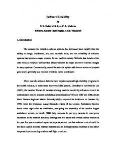
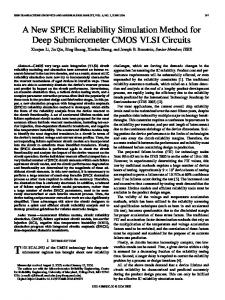
306  2 Total Predicted Faults, 252  45 Days

250 200 F a u 150 l ts

Operations Transfer

100 50 0

0

Preliminary 50

100 150 200 Test Days Figure 16-1: Faults vs. execution time in test and operational facilities for a system of about 100,000 lines of assembly-language code. Figure ?? illustrates the eects that environment can have on the test pro le. It depicts best- t curves to actual cumulative failure data taken over three portions of a test activity. The software under test was part of the ground data system used in NASA's deep-space missions. The testing marked \Preliminary" was preparatory in nature, performed while the software was being installed in a \compatibility test area," or test facility con gured to match identically the operational environment to the extent economically feasible. The facility contained essentially everything electronic except the large-aperture antennas, low-noise maser receiver ampli ers, high-power transmitters, and spacecraft data system, that the later operational environment would have. Interfaces with missing operational subsystems were simulated. Testing during the pre-transfer period proceeded until the failure rate leveled o at about 200 total faults (a predicted 18 faults remained). Then, activity transferred to deep-space tracking stations using similar scenarios, but in operational situations. Testing during this period found another 95 faults (considerably more than the 18 predicted). Despite the fact that the con gurations and scenarios were essentially identical, there were about 306 ? 218 = 88 faults that would never have been found had testing continued only in the test facility! Predicting failures in diering environments requires, at the least, adaptability of the reliability model to t con guration, scenario, and previous failure data. Such adaptations must accommodate for dierences in hardware, test strategies, loading, database volume, and user training.

4 ARTIFACT-BASED SIMULATION

Software developers have long questioned the nature of relationships between software failures and program structure, programming error characteristics, and test strategies. Von Mayrhauser et al. [?, ?, ?] have performed experiments to investigate such questions, arguing that the extent to which reliability depends merely on these factors can be measured by generating random programs having the given characteristics, 6

and then observing their failure statistics. It is not important, in this respect, that the programs actually execute to perform useful functions, but merely that they possess the hypothesized properties that \real" programs would have in a given environment. If the hypothesis is true, then the eects of the various controlled elements under study would be readily discovered. For example, by adjusting code structural characteristics (e.g., size, ratio of branching decisions to loop decisions, and fault distribution) in a controlled set of experiments, one may observe the contributory eects to failure behavior. One may also learn something about the sensitivities of reliability models to their founding assumptions. Such studies would lead practitioners to the best model(s) to use in given situations. To explore the conjecture, they identi ed program properties and test strategies to be investigated. Then they performed experiments using automatically generated programs having the given properties, subjected these to the selected test strategies, and measured the reliability results. Their investigations proceeded using only single-module programs (i.e., ones with no procedure calls), assumed that faults are only of a single type and severity, distributed uniformly throughout the program, and considered only a constant likelihood that a failure results when execution encounters a statement containing a fault. There is no fundamental limitation in the artifact simulation technique that excludes procedure calls, multiple fault types, and time-dependent statistics. They were excluded in these early experiments to establish basic relationships. Their architecture will support multiple subprograms, faults of various types, severities, and distributions, and time-varying parameters at the later stages of experimentation.

4.1 Simulator Architecture

The reported simulation covers the coding, testing, and debugging portions of the software life cycle. The simulator consists of the following components (see Figure ??). Code Generator

Test Data Generator

?

Compiler

?

-

Test Harness

-

6

Reliability Analysis 6

-



Test Report

 

?

Code Repair



Debugging

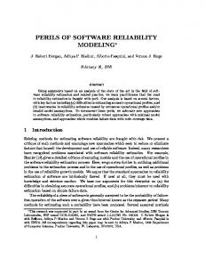
Figure 16-2: Artifact-based software process simulator program. The Code Generator uses program design and/or code structural and error characteristics to produce executable code with faults. Code generation is discussed more fully later (Section 16.??). The faults injected into the program cause actual execution failures during testing to occur in such a manner as to be detected by the Test Harness module, discussed below. The Compiler is an ordinary compiler, the same as an actual project would use. The compiler generates executable code from the generated code and from updates following each of the fault repairs. The Test Data Generator uses the generated code, together with parameters that select testing strategy, testing criteria, and phase (unit test, integration test, system test, etc.) to produce test input data and testing procedure parameters. The Test Harness module applies test data to the simulated system in accordance with the selected test procedures, then detects each failure as it occurs, and categorizes it according to predetermined fault exposure and severity criteria. 7

The Debugger and Code Repair function of the simulation locates and repairs faults recognized by the test harness, and then reschedules the program for compilation and retesting. The debugger may fail to locate the fault and may either completely or incompletely remove the fault, when located. It may, at times, even introduce new faults. The debugger parameters include inputs to control locatability, severity, completeness, and fault detectability. Reliability Analysis combines the failure data output by the test harness with the residual fault data from the debugger (undetected errors and incorrect repairs) to assess the reliability of the simulated code. This assessment compares failure results with the output of a conventional software reliability model.

4.1.1 Simulation Inputs

Artifact simulation experiments can vary many aspects of program construction and testing to investigate the eect of static properties on dynamic behavior. Inputs may include those which characterize code structure, coding errors, test input data, test conduct, failure characteristics debugging eectiveness, and computing environment. The investigated code structure parameters pertained to control ow, data declaration, structural nesting, and number and size of subprograms. Statement type frequencies represented the structural dependencies of a program. The experiments assumed four types of program statements: assignments, looping statements, if statements, and subprogram calls. Data structure declaration characteristics were not simulated because faults in such structures tend to be caught by the compiler, and because the eects of faults in such statements would be included among those of the four chosen types. Type, distribution, density, and fault-to-failure relationship parameters in uenced the insertion of coding errors. The generator used type information to select the kinds of statements composing the program. Distribution information controlled where faults were located, either clustered in speci ed functions or scattered randomly throughout the program. Fault-to-failure relationships de ned the frequency of failures when faults are encountered at run time. Test input data depend on the testing environment, operational scenario, testing strategies, test phase, desired coverage, and resources available for testing. In the simulations reported, resource considerations were not addressed. Provisions for test strategies included features for random, directed, functional, mutation, sequencing, and feature testing. Test coverage selection included parameters designating node, branch, and data ow modes. Projects classify failure attributes by type, severity, and detection status. Investigations so far have treated only failures of a single type and severity. Debugging eectiveness depended on parameters associated with fault detection, identi cation, severity, and repair. Each of these, except severity, has correctness and resource dimensions. For example, identi cation establishes a fault-to-failure correspondence and the time required to make that correspondence. Computing environment parameters included all the data required to run the test harness and analyze the failure data. The experiment environment data included machine, language, and workload parameters.

4.1.2 Simulated Code Generation

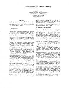
A code generator may produce simulated code using measured parameters of the actual project (trace-driven), or from generic data taken from a wide variety of project histories (self-driven). Figure ?? illustrates a self-driven code generator architecture. The reported code simulator operates approximately as follows: Given the number of modules and the set of module sizes, the generator creates statements of the speci ed types according to their given occurrence frequencies, sometimes followed by code that represents a fault of the a speci ed character. The means for invoking multiple modules and for controlling the depth and length of nested structures were not explicitly revealed in the source references. Readers wishing to duplicate the simulator for their own experiments will have to decide upon appropriate models for these characteristics. It is not necessarily assumed that real faults are uniformly distributed over the program; rather, the program generator can seed faults either on a function-by-function basis or statement-by-statement, according to a distribution by statement type and nesting level. Further, the fault exposure ratios of each fault need not be the same. 8

#

#

"

!"

Statement Type Frequencies

Fault Density

?

Statement Type Selection

!

?

-

Fault Insertion

   

6

Generated Program Statements

   

6

Random Number Generator

Figure 16-3: Self-driven artifact simulation of the coding phase. The presence of a real fault in a normal program corresponds to an ersatz element within the simulated program that can cause a failure contingent on a supposed failure characteristic. As the simulated program executes, a statement containing a fault will, with a given probability (the fault exposure ratio), cause a failure. But the ersatz failure, when it occurs, is is not meant to duplicate the appearance the real failure; only its occurrence and location are of importance. The injected fault thus needs to raise an exception with information that will identify where, when, and what type of failure has occurred. The reported simulator used a divide-by-zero expression to trigger the fault, which was then trapped by the execution harness via the signal capability of C. An important step toward extending the utility of the simulation technique would be to make it tracedriven, or adaptive to project measurements as they emerge dynamically, rather than using only the static historic data of the self-driven simulation described above. Figure ?? illustrates how trace data would replace the random selection of statements during program execution.

4.1.3 The Execution Harness

The reported execution harness contains a test driver program that creates an interface between the generated program and its test data, spawns a \child" process to execute the generated program, and collects executiontime data on the child process separately from that of its ancillary functions, which may not have the same structural characteristics. The returned value of the child process indicated whether the test resulted in failure, or terminated naturally. Simulated faults in the generated program could have been represented in any of a number of ways. The reported experiments used arithmetic over ow. Having detected the failure, the test harness enters the returned information into the failure log for use in locating and removing the fault. The updated program then recompiles and re-executes.

4.1.4 Reliability Assessment

The output log provides the execution time of each test run and indicates which runs experienced failures; it also identi es which fault caused the failure. Tools, such as those described in Appendix A, can use this data to generate tabular and graphical analyses of the failures. Such analyses may include application of any of a number of reliability growth models, maximum likelihood estimates and con dence limits for model parameters, and visual plots of important reliability attributes, such as cumulative failures or present failure intensity versus time. 9

#

Project PDL

"

?

PDL Analyzer

! #

Fault Density

"

?

Statement Type Selection

!

?

-

Fault Insertion

   

Generated Program Statements

   

6

Random Number Generator

Figure 16-4: Trace-driven artifact simulation of the coding phase. The reliability assessment function also has available to it the output of the debugging function, which tells which faults were correctly, incorrectly, or incompletely made. At any time, then, the status of remaining faults in the generated program is visible.

4.2 Results

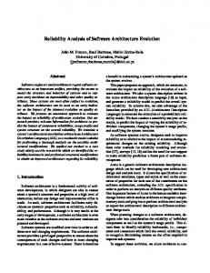
Reliability investigations using artifact simulation are currently in their formative stage. The fundamental, rst-order validations of the equivalence hypotheses are yet in progress. Consequently, the process of evolution has imposed some limitations that will disappear, with time. The fundamental question has been: Do simulated programs in simulated environments exhibit reliability pro les representative of \real" programs in \real" environments that have the same parameters? A software artifact simulation study, [?], compared (Figure ??) the results of testing a 5000 line C program with the predicted performance using the basic execution time model. These experiments demonstrated that the order in which failures occurred among statements containing faults closely matched the execution counts for those statements, and that the failure counts correlated with the types of program structures surrounding the faults. These and other early results tend to con rm that static measures of program structure, error characteristics, and test strategies in uence the reliability pro les of simulated and \real" programs in the same ways. (Mike: TBD The reviewer asked \Can you relate this artifact-based simulation to work on FINE (at Univ of Illinois?) or other such fault-injection methods and tools?" Do you know of this work, and can you supply the information asked for?) Artifact simulation studies of the future will continue to quantify the extent to which static parameters relate to reliability dynamics. As the software simulation art evolves, the eects of size, multiple-procedure program structures, multiple failure types, nonuniform fault distributions, and nonstationary parameters on reliability will increasingly become known.

10

F a i l u re s

20

10

0 0.00

0.10 0.20 Execution Time (CPU hrs) Figure 16-5: Simulated code experimental cumulative failures (from [Mayr91]).

5 RATE-BASED SIMULATION

The fundamental basis of rate-controlled event process simulation is the representation of a stochastic phenomenon of interest by a time series x(t) whose behavior depends only on a rate function, call it (t), where (t) dt acts as the conditional probability that a speci ed event occurs in the in nitesimal interval (t; t + dt). A number of the analytic reliability growth models discussed in Chapter 4 echo this assumption and further assume that events in non-overlapping time intervals are independent. The processes modeled are thereby Markov processes [?], or non-homogeneous Poisson processes (NHPP), which are also Markov processes. These include the models proposed by Jelinski and Moranda ([?]), Goel and Okumoto ([?]), Musa and Okumoto ([?]), Duane ([?]), Littlewood and Verrall ([?]), and Yamada ([?]). Rate functions for these appear in Section 16.??. The algorithms described here not only apply to simulating Markov processes, but are capable of simulating processes having time-dependent event count dependencies and irregular rate functions. These algorithms can simulate a much more general and realistic reliability process than has ever been hypothesized for any analytic model. The mathematics presented in this Section treat general statistical event processes and rate-driven event processes, not merely those believed to describe software failures. As in the analytic models mentioned above, it is only the form of the rate functions and interpretation of parameters that set these models apart as pertaining to software. We begin this specialization formally in the next Section and continue it through Section 16.??. First, however, we derive the forms of the simulation algorithms.

5.1 Event Process Statistics

If S0 and S1 denote the states of an event E, S0 in eect before the event and S1 after its occurrence, then a particular member of the stochastic time series de ned by f 0 (t); S0 ; S1 g beginning at time t = 0 is a sample function, or realization, of the general rate-based discrete-event stochastic process. The zero subscript on 0 (t) signi es the S0 , or zero occurrences, starting state. The statistical behavior of this process is well-known: The probability that event E will not have occurred prior to a given time t is given by the expression 11

where

P0(t) = e?0 (t; 0) (t; t0 ) =

Z

t t0

0 () d

(16-1) (16-2)

The form of 0 (t) is unrestricted, but generally must satisfy 0 (t)  0 and 0 (1; 0) = 1 (16-3) The rst of these prevents the event from occurring at a negative rate, and the second stipulates that the event must eventually occur. If the second condition is violated, there will be a nite probability that the event will never occur. When the events of interest are failures, 0 (t) is often referred to as the process hazard function and 0(t; 0) is the total hazard. The probability distribution function and probability density for the time of an occurrence are then F1 (t) = 1 ? P0(t) f1 (t) = 0 (t)e?0 (t; 0) The mean time of occurrence is

E(t) =

Z

1

0

t 0 (t) e?0 (t; 0) dt

(16-4) (16-5) (16-6)

If 0(t; 0) is known in closed form, we may sometimes be able to write down and analyze the event probability and mean time of occurrence functions directly. In all but the simplest cases, however, we will require the assistance of a computer. When we cannot express the integrals in closed form, we can still evaluate them using straightforward numerical analysis.

5.2 Single-Event Process Simulation

It is rather easy and straightforward to simulate the rate-based single-discrete-event process, as illustrated in the following computer algorithm (expressed in the C programming language) which returns the occurrence time: double single_event(double t, double dt, double (*beta)(double)) { int event = 0;

}

while (event == 0) { if (occurs(beta(t) * dt)) event++; t += dt; } return t;

Above, the C language syntax de nes a function named single event() that will eventually return a -precision oating-point value of the time of event occurrence. Starting at time t, and continuing as long as the event value remains 0, the function monitors the event status; at the occurrence, event increases by 1, as signi ed by the ++ operation, which stops the iteration. Time augments by dt units each iteration, denoted by the \+=" operation. We have programmed the occurs(x) operation as a macro that compares a random() value over [0; 1) with the formal parameter x, which must be less than unity, thus attaining the speci ed conditional probability function. (The extern double designation declares that random() is in an external library that returns a double precision oating-point value.) The interested reader may wish to consult [?] for a discussion of random number generation techniques. double

12

extern double random(void); #define occurs(x) (random() < x)

The particular application determines the form of the user-supplied rate function beta(t). Any required initialization takes place in the main() program prior to invocation of the single event() function. Figure ?? depicts the basic data ow of the overall program.

#

System Parameters

-

initialize()

"

!

?

6

Rate Function

-

beta(t)

?

main()

-

Simulation Algorithm

single event()

-

t

Figure 16-6: Simulation program structure for a single event occurrence. We must choose the dt in simulations to satisfy the following conditions: 1. dt is smaller than the desired time-granularity of the reliability pro le, 2. variation in (t) over the incremental time intervals (t; t + dt) is negligible, 3. the chance of multiple event occurrences within a dt interval is negligible, and 4. the magnitude of (t) dt is less than unity at each t in the interval of interest. The time-complexity of the algorithm is O( t=dt), where the component represents the maximum complexity of computing (t). We may also simulate the behavior of a non-stochastic3 rate-based single-event process merely by altering the algorithm for occurs(). If (t) represents the occurrence rate, then the event occurs when its integral reaches unity. double accumulated_rate; #define occurs(x) (if ((accumulated_rate += x) < 1.) \ then FALSE else TRUE)

The construction above increments accumulated rate by x prior to checking its value; the expression then switches from a false to a true state when the value reaches unity. (The \\" at the end of the line signi es continuation on the next line of the macro.)

5.3 Recurrent Event Statistics

If we permitted the iteration in the previous algorithm to continue throughout a given time interval (0; t), then the simulated event could occur a random number of times, which could be counted. We may compute the probability distribution function Fn(t) that the n occurrence lies in the interval (0; t) as follows: If tn?1 has just been observed as the (n ? 1)st event occurrence, then we may treat the interval immediately after tn?1 as a new experiment. Translating Eq. (??) to the nth occurrence interval produces the occurrence distribution function conditioned on tn?1, 3 This technique also approximates the calculation of the mean occurrence behavior of a stochastic process; however, the method is exact only for the constant hazard case.

13

Pn?1(t j tn?1) = e?n?1 (t; tn?1 ) Fn(t j tn?1) = 1 ? Pn?1(t j tn?1) Z

k (t; tk ) =

t

tk

k () d

(16-7) (16-8) (16-9)

The time dependency retained in Eq. (??) re ects the possible nonstationary nature of the event process. Each of the k (t) functions is subject to the restrictions given in condition (??); otherwise Fn (t j tn?1) above must be divided by 1 ? Pn?1(1 j tn?1) = 1 ? e?(1; tn?1 ) . We shall assume these requirements in the remainder of this Chapter. The n th occurrence probability densities then follow from dierentiation of Eq. (??), fn (t j tn?1) = n?1 (t) e?n?1 (t; tn?1 ) Z t fn(t) = n?1 (t) e?n?1 (t;  ) fn?1() d 0

(16-10) (16-11)

the latter being recursively de ned, with t0 for the n = 1 case de ned as 0. The conditional probability displays the same type of statistical behavior seen in Eq. (??) for the single occurrence case above, but operates piecewise on successive intervals between occurrences. Finally, Fn (t) follows by integration, Fn(t) =

Z

t

0

fn () d

(16-12)

When events are modeled as Markov occurrences, the probability Pn(t) that exactly n occurrences appear in the interval (0; t) is known [?] to be of the form P0(t) = e?0 (t; 0)

(16-13)

Pn(t) =

(16-14)

Z

t

0

n?1 Pn?1 e?n (t;  ) d

Mathematically closed-form solutions for these probability functions are rarely4 known. General solutions thus require simple, but perhaps time consuming, recursive numerical methods: The time-complexity of fn (t j tn?1) is of order O( (t ? tn?1)=dt); fn (t) and Pn(t) are of order O( nt=dt), and Fn(t) is also of order O( nt=dt). The space complexities of these measures are, respectively, O(1), O(t=dt), and O(t=dt). The expected time of the n th occurrence follows directly from Eq. (??) as a recursive expression, tn =

Z

0

1

t n?1(t)

Z

t

0

e?n?1 (t;  ) fn?1 () d

(16-15)

with time-complexity O( nt1 =dt) and space complexity O(t1 =dt).

5.4 Recurrent Event Simulation

Simulation oers a relatively economical alternative in the evaluation of rate-based performance over the more complex numeric integrations of the previous Section. The recurrent events algorithm below is a simple extension of the single-occurrence event code that returns the number of occurrences over the time interval (ta ; t). Its computational complexity to the nth occurrence is only O( tn =dt), in constant space: 4 Closed-form solutions for P (t) and f (t) are known to exist when the process is of the non-homogeneous Poisson variety, n n namely Pn (t) = n (t; 0)exp[?(t; 0)]=n! and fn (t) = (t)n?1(t; 0)exp[?(t; 0)]=(n ? 1)!.

14

void recurrent_event(double ta, double t, double dt, double (*beta)(int, double), int *events) { while (ta < t) { if (occurs(beta(events, ta) * dt)) ++*events; ta += dt; } }

The calling program must initialize the events parameter to the actual number of occurrences prior to time ta ; events will contain the new count after the function returns. (Note that we renamed events in the plural to acknowledge that multiple occurrences are being counted.) Figure ?? depicts the program data ow structure.

#

System Parameters

-

"

initialize()

!

?

Rate Function

-

6

beta(e, t)

?

main()

Simulation Algorithm

-

recurrent event()

-

events

Figure 16-7: Simulation program for recurrent events. Mathematically, n (t) is valid only in the interval tn  t < tn+1 and signi es that n occurrences of the event have occurred prior to t. The use of beta(events, t) in the algorithm acknowledges that the event may recur from time to time and that the occurrence rate function may not only change over time, but also may be sensitive to the number of event occurrences (as well as possibly other in uences). The simulation algorithm observes the event occurrence times and may change the beta() function as required by the application. We may also simulate non-stochastic rate-based recurrent-event processes5 by making the single-occurrence occurs() function recognize unit crossings of the rate accumulator, as follows: #define occurs(x) (if ((accumulated_rate += x) < 1.) \ then FALSE else (accumulated_rate -= 1., TRUE))

Note that accumulated rate decrements by unity at each occurrence, signi ed by the \-=" operation.

5.5 Secondary Event Simulation

Another type of event process of interest is when a primary event triggers the occurrence of a secondary event of a dierent type. For example, producing a unit of code may create a fault in the code. Notationally, if pi denotes the probability that the ith occurrence of the primary event causes the occurrence of the secondary event, then we may express the probability Pm(2)(t) that m such secondary events have occurred in the interval (0; t) as Pm(2)(t) =

1 X

pmjn(t)Pn (t) n=m 5 This technique, as before, approximates the average occurrence behavior of stochastic recurrent-event processes. 15

(16-16)

with pmjn = Probfm secondary eventsjn primary events in (0; t)g X pi1 : : :pim (1 ? pim+1 ) : : :(1 ? pin ) = i2I

(16-17) (16-18)

where the index vector i = (i1 ; i2 ; : : :; in) is a permutation of?(1;
2; : : :; n) such that (i1 ; : : :; im ) extends over all combinations of m out of n primary events, a set I of size mn . The computational complexity of Pm(2)(t) is thus of combinatorial order, and not practical to evaluate in general cases of practical interest. In the special case that pi = p is constant, pmjn reduces to the binomial function,   n pm (1 ? p)n?m (16-19) pmjn = m The simulation algorithm for a dependent secondary event process, however, can remain quite general; one merely adds a mapping array secondary event that relates the primary event to its secondary event and a function p(i, events, t) that returns the probability that the primary event triggers the secondary event. if (occurs(beta(i, events, ta) * dt)) { ++events[i]; if ((j = secondary_event[i]) && occurs(p(j, events, t))) { ++events[j]; } }

We may similarly treat multiple secondary events emanating from a single primary event, at only a moderate increase in algorithm complexity.

5.6 Limited Growth Simulation

When the nal number N of occurrences that an event process may reach is prespeci ed, the normal growth of the event count over time must stop after the Nth occurrence. For example, if there are N faults to repair and repairs proceed reasonably, then eort ceases after the last one is xed. Simulating this behavior is simple, but must include steps to prevent the event count from overshooting N when multiple occurrences occasionally take place within a dt interval. This may be done by altering the event counting functions not to exceed prespeci ed maxima max events as follows: if (events[i] < max_events[i]) ++events[i];

5.7 The General Simulation Algorithm

You may have already guessed the form of a general rate-based discrete-event process simulator. It is merely the recurrent-event algorithm augmented to accommodate multiple simultaneous events, multiple event categories, secondary events, and growth limits. The general algorithm below incorporates all of these features. It simulates f event processes over a time interval ta to t using time slices of duration dt; an initialized input array events counts the occurrences, which may not exceed corresponding values in the max events array; an array event categories contains the mapping of event occurrences into categories, which counts occurrences up to the maxima speci ed in the max categories array; and a secondary event array and p() function control secondary occurrences, as described in Section 16.??. For readability, the control function name beta() becomes rate(). We also add action() and display() functions, described below. void simulate(int f, double ta, double t, double dt, double (*rate)(int, int *, double), int events[ ], int max_events[ ], int categories[ ], int max_categories[ ], int event_category[ ], int secondary_event[ ], double (*p)(int, int *, double),

16

void (*action)(int *, double), void (*display)(int *, double)) {

int i, j, k; while (ta < t) { for (i = 0; i < f; i++) { if (occurs(rate(i, events, ta) * dt)) { if (events[i] < max_events[i]) { ++events[i]; k = event_category[i]; if (categories[k] < max_categories[k]) ++categories[k]; } if ((j = secondary_event[i]) && occurs(p(j, events, ta)) { if (events[j] < max_events[j]) { ++events[j]; k = event_category[j]; if (categories[k] < max_categories[k]) ++categories[k]; } } action(events, ta); } } ta += dt; display(events, ta); }

}

The action() function speci es what takes place when an event occurs. For example, if one category of events represents identi ed faults and another represents repairs, then action() may compute an unrepaired fault parameter for display(), or it may recompute appropriate max events or max categories bounds. The action() functions may well also pass additional parameters, such as i, j, k, and m, should these local values be needed to eect the proper change in state. The display() function outputs the simulation status monitors as a pro le in time. It may publish only certain parameters of interest, or it may detail the entire reliability state at each dt, depending on the time-line information desired by the user. Figure ?? shows the overall simulation program data ow.

# -

initialize()

System Parameters

"



!

?

6

-

Rate Function

rate(i, e, t)

action()

6 ?

main()

-

Simulation Algorithm

 -

simulate()



 

display()

 

 

Figure 16-8: General rate-controlled process simulator program. We must choose the dt for the simulation experiments simultaneously to satisfy earlier-stated constraints imposed by each of the event rates. As a consequence, execution may be very slow. Alternatively, we could speed up the algorithm by choosing larger values of dt and computing the numbers of multiple events that may occur during each of the larger intervals, as determined by the probability functions of primary and 17

secondary events. It is known, when event occurrences in non-overlapping intervals are independent (see, e.g., [?]), that primary events are Poisson distributed and secondary events are binomially distributed. Generally, however, the probability functions are unknown, even when the rate functions are fairly simple. But if these probability functions were known, there would only be slight changes required in the algorithm above: occurs(rate() * dt) would be replaced by a primary(rate() * dt) function that counts the random number n of primary event occurrences in the dt interval; occurs(p()) gets replaced by secondary(n, p()), which counts the number m of occurrences of secondary events; and events[] augments by n and m, rather than unity, respectivly. If we desire, for execution-time reasons, a value of dt that is too large for use in the general algorithm above, but is yet small enough that primary and secondary event statistics over dt intervals are approximately Poisson and binomially distributed, respectively, then the modi ed algorithm can be applied. We refer to this con guration as the \piecewise-Poisson" approximate simulation. Piecewise-Poisson simulations, of course, are valid for the all the usual NHPP models, because no approximations are actually made. We have not yet studied the validity of the approximation applied to other processes.

6 RATE-BASED RELIABILITY

Rate-based reliability simulation is a natural extension of techniques for analyzing conventional models, because many of these are also are rate (or hazard) based. The underlying processes assumed by these models are thus the same. Because of algorithmic simplicity, simulation serves as a powerful tool not only for analyzing the behaviors of processes assumed to have complex rate functions, but also for investigating whether the stochastic nature of a project's measured failure data is typical of that obtained by simulation. One may vary the modeling assumptions until pro les reach a satisfactory alignment. The challenge in life cycle simulation is nding rate functions that satisfactorily describe all of the activities, not just testing. Such a model enables optimum planning through trade-os among allocated resources, test strategies, etc.

6.1 Rate Functions of Conventional Models

Several published analytic models treat (or approximate) the overall growth in reliability during the test and fault removal phases as non-homogeneous Poisson processes in execution time, while others focus on Markov execution-time interval statistics. While these may dier signi cantly in their assumptions about underlying failure mechanisms, they dier mathematically only in the forms of their rate functions. Some examples are the following: 1. The Jelinski-Moranda model [?] describes statistics of failure time intervals under the presumption that n (t) = 0 (1 ? n=n0), where n0 is the estimated (unknown) number of initial software faults and 0 is initial failure rate. 2. The Goel-Okumoto model [?] treats an overall reliability growth process with (t) = n0e?t , where n0 and  are input parameters, n0 being the initial failure rate, and  the rate decay factor. Strictly speaking, this rate function violates the conditions on (t; 0) imposed in (??), because 0 (1; 0) = n0 and P0(1) = e?n0 . In practicality, n0 is usually fairly large, so the consequences may be negligible. 3. The Musa-Okumoto model [?] posits an overall reliability growth process in which (t) = 0 =(1+t), where 0 is the initial failure rate and  is a rate decay factor. Both 0 and  are input parameters. 4. The Duane model [?] deals with another overall reliability growth model, with (t) = kbtb?1, where k and b are input parameters. Condition (??) requires that 0 < < 1. 5. ThepLittlewood-Verrall inverse linear model [?] is an overall reliability growth model with (t) = 0 = 1 + t where 0 is the initial failure rate and  is a rate decay factor. 6. The Yamada delayed S-shape model [?] represents still another overall reliability growth model, with (t) =  te1? t , where  (the maximum failure rate) and are input parameters. This rate function, 18

too, violates condition (??), as 0 (1; 0) = e= and P0 (1) = e?e= ; again, when the large number of faults is large, the eect is negligible. You may nd discussions of these models elsewhere in Chapter 4.

6.2 Simulator Architecture

We have already discussed the algorithm for rate-based simulation. The remaining architectural considerations are characterized by input parameters, event rate functions, event-response actions, and output displays. The scope of user requirements should set the level of detail being simulated. A reliability process simulator should be able to respond to schedules and work plans and to report the performance of subprocesses under the plan. By viewing simulated results, users may then replan as necessary. The simulator described here therefore does not assume speci c relationships involving sta, resource, or schedules, but expects these as inputs, in the form described in Section 16.??. Simulations should also embody interrelationships among project elements. For example, defective speci cations should lead to faults in the code unless defects are corrected before coding takes place; missing speci cations should introduce even more coding errors; testing should not take place without test cases to consume; repair activity should follow fault identi cation and isolation; and so on. A more comprehensive simulation model ([?]) of the reliability process uses about 70 input parameters describing the software project and development environment, together with a project plan of arbitrary length containing activities, resources allocated, and application schedules. This simulator displays time-line pro les of almost 50 measures of project reliability status and the resources consumed, by activity. Its experimental use is described later in Section 16.??. We shall illustrate the principles of reliability process simulation in a somewhat more simpli ed example| only 25 input parameters and a project resource schedule are required. You should not regard this example necessarily as a tool ready for industrial use, but as a framework and means for experimentation, learning, and extension. In the example, we simulate only a single category of events for each reliability subprocess. Further, simulations produce only two types of failure events, namely, defects in speci cation documents and faults in code, all considered to be in the same severity category. We also simplify the example reliability process not to include document and code reuse and integration, test preparations and the dependencies between testing and test-case availability, outages due to test failures, repair validation, and retesting. Other, more detailed, simpli cations appear in the discussions below.

6.2.1 Environment Considerations

We know that characteristics of the programming, inspection, test, and operational environments can in uence the rates at which activities take place. For simplicity, however, we have eliminated as many of these from the example simulator as seemed reasonable to our goals here. A more re ned tool for general-purpose industrial use would, of course, probably include more de nitive environmental inputs. Events, of themselves, carry no intrinsic hazard values. The rates at which events occur depend on a number of environmental and other factors, including the nature of the events themselves. The model must treat event hazards dierently in dierent situations. Some faults may be easier to discover by inspection than by testing, while for others, the opposite may be true. The fault discovery rate in testing normally depends on such parameters as the CPU instruction execution rate, the language expansion factor, the failure-to-fault relationship, and the scheduled CPU hours per calendar day that are applied. During inspections, on the other hand, fault discovery depends on the discovery-to-fault relationship, the fault density, the inspection rate, and applied eort. A fault is independent of its means of discovery. The model must therefore realize dierent hazard-perfault rates in diering discovery environments, rather than merely assign a speci c hazard rate to the fault itself.

19

6.2.2 Subprocess Representation

In the example simulator, each activity produces occurrences of one or more uncategorized event types, either primary or secondary. Table ?? lists the simulated primary events. Except for test failures, all are goal-oriented processes with limiting values, as shown. Test failures are limited by the current fault hazard function. Table 16-1: Reliability process primary events and limits. Primary Event doc unit created doc unit inspected doc defect treated code unit created code unit inspected code fault treated test failure failure analyzed fault repair attempt

Rate Control build workforce document insp workforce document corr workforce coding workforce code insp workforce code corr workforce size, faults, cpu, exposure analysis workforce repair workforce

Limit doc size doc insp goal defects recognized code size code insp goal faults created

1

test failures faults found

Table ?? de nes the secondary events that occur with a primary event, controlled by an occurrence probability that may depend on a number of combined factors. For example, the number of defects or faults recognized during inspections will not only depend on the inspection eciency (the fraction of defects recognized when inspected), but also on the density of defects in the material being inspected. All secondary event occurrences are naturally limited in number to the occurrences of their primary events; no other limits are imposed. Table 16-2: Reliability process secondary events, correspondences, and controls. Secondary Event Primary Event Rate Control defect created doc unit created defect density defect recognized doc unit inspected latent defects, eciency defect corrected defect treated correction eciency fault created code unit created fault density, missing/faulty doc fault recognized code unit inspected latent fault density, eciency fault corrected fault treated fault correction eciency test failure fault identi ed failure analyzed id eciency, fault density fault repaired repair attempt repair eciency

6.2.3 Document Construction

Document generation occurs presumably at a constant mean number of units per workday, not to exceed the document size goal, modeled as a Poisson random value whose mean is the given size. Defects occur at a constantaverage rate per produced unit. The general simulation algorithm requires that the average number of defects committed per dt interval be made less than unity by choice of dt. For example, if one chooses the documentation unit as the page, then there should be fewer than one defect in the number of pages produced in the time dt, on average. If one expects a greater defect rate, then a smaller dt must be chosen. (Use of the piecewise-Poisson approximation model would relax this restriction to the dt over which the approximation is valid). Input parameters are 20

doc_size doc_per_workday defects_per_unit

6.2.4 Document Inspection

Document inspection is a goal-limited process similar to document construction. Inspections take place at constant average rates per workday, encountering defects in proportion to the defect density and applied inspection eort, but recognizing only a fraction of those defects encountered. The number of inspected units at any time may not exceed the number of units so far created, nor the document inspection goal, a binomially distributed value determined from the document size goal and the input inspection fraction. The number of defects recognized cannot, of course, exceed the number created. Because known defects may not yet have been removed at the time of an inspection discovery, we count the event as a new defect in proportion to the fraction of as-yet undiscovered defects. The salient input parameters are doc_inspection_fraction doc_inspected_per_workday fraction_defects_recognized

6.2.5 Document Correction

Sta resources, correction resource requirements per defect, and defect correction eciency determine the rate at which defects get treated and thereby corrected. Attempted corrections may also inject new defects. Corrections decrease the defect count, while new defects increase it. The number of defects treated at any time is less than the number so far recognized, plus the number of bad corrections (i.e., defects treated but not corrected). The number of corrections cannot exceed either the number of defects recognized or treated. Generally, defect corrections could change the overall amount of required documentation; however, we have not modeled this eect here. The input values needed are defects_treated_per_workday fraction_defects_fixed

6.2.6 Code Construction

Code production follows the same general routine as document construction. However, the faults injected depend not only on normal human fallibility, but also on the amount of defective and missing speci cations, all three of which could cause faults of dierent classi cations. We assign each injected fault in the example simulator to the same category, however. As with documentation, we must assure that the number of faults per dt interval not exceed unity over the duration of interest. For example, if one chooses the code unit as a line of code, then there should not be more than one fault injected into the number of lines of code produced in dt time units, on average. The number of units created is limited by the code size goal, a Poisson-distributed value whose mean is the input size. External inputs required are code_size code_per_workday faults_per_unit faults_per_defect faults_per_missing_doc_unit

Fault injection is a secondary event to code unit construction; the number of faults per code unit has three sources: the faults per code unit produced from perfect speci cations; faults per document defect times the average number of defects per unit code; and the faults per missing document unit times the number of missing documentation units per code unit. 21

6.2.7 Code Inspection

Code inspection mirrors the document inspection process. Inspections take place at constant average rates per workday, encountering faults in proportion to fault density and applied inspection eort, but recognizing only a fraction of those encountered. The number of units inspected cannot exceed the number of code units created so far, nor the code inspection goal, a binomially distributed value determined from the code size goal and the input inspection fraction. The number of faults recognized, of course, cannot exceed the number injected. External input values are code_inspection_fraction code_inspected_per_workday fraction_faults_recognized

Since previously found faults may not yet have been removed at the time of an inspection discovery, we count a fault discovery as a new fault in proportion to the fraction of as-yet undiscovered faults.

6.2.8 Code Correction

Code correction simulation follows the document correction pattern, translated to code units. Fault correction attempts reduce the open fault count when successful and may increase it if unsuccessful. The number of faults treated cannot exceed the number recognized, plus the number treated but not xed. The number of faults corrected is limited to the number found by inspection and the number treated so far. In general, code corrections may require document changes. The simulator consumes resources for such changes, but does not alter the documentation size and defect status. The input parameters that apply to code correction are faults_treated_per_workday fraction_faults_fixed

6.2.9 Testing

In simulated test activities, failures occur in proportion to the test hazard per fault, the current fault density, and applied CPU resources. The resource schedule speci es the rates of CPU consumption, so the only additional input parameters needed is test_hazard_per_fault

The test hazard per fault parameter depends on the CPU execution rate, the compiler code expansion factor, and the fault exposure ratio. The number of test failures is unlimited; as long as there are faults, failures will occur at the hazard rate.

6.2.10 Fault Identi cation

The simulator presumes that projects analyze failures at constant average rates per workday, not to exceed the number of failures observed. The number of faults identi ed must remain less than the number created, but unrecognized by inspection. The fraction of undiscovered faults and the probability of correct isolation regulate the fault identi cation process. Pertinent inputs are failures_analyzed_per_workday fraction_failures_isolated

22

6.2.11 Fault Repair

Attempts to remove faults consume constant average resources per fault. Only a fraction of attempted repairs are actually successful; the rest will mistakenly be reported as repaired. The number of attempted repairs cannot exceed the number of faults so-far found (in inspections, as well as in testing), plus the number bad repair attempts (those that did not result in fault removal). The number of faults removed in this process must not exceed the number found, less those that were corrected after inspections, and also may not exceed the number of repair attempts. Resources consumed by attempted code repairs include resources for changes in code and documents. The amounts and makeup of code and documentation do not change, however. Input parameters are code_repairs_per_workday fraction_faults_repaired

6.3 Display of Results

Internally, a process simulator carries very detailed, ne-grained information on the activities and events under study, of types that are both visible and latent in real projects. In the spirit of simulation, the pro les viewed by humans should appear as if taken from reality. However, a simulation user may well desire visibility into latent values, such as the numbers of unfound defects and faults, in order to make decisions on subsequent actions. When real project pro les match their corresponding simulation pro les, then the user probably expects that the latent behaviors will also agree. But one must not expect latent, model-internal behaviors to be accurate, because they can never be matched with reality. To some extent, real pro les depend on how projects instrument and organize themselves for reliability measurement. They may record the status of documents and development code only at certain milestones. Other parameters, such as failures, may be logged automatically by the operating system, if detected, or by humans on a daily or weekly basis. Visible project parameters include (1) the input facts (or assumptions) that de ne the environment and (2) the measured pro les, such as pages of documentation, lines of code, defects and faults found by inspections, failures, test faults identi ed, repairs, resources expended, and schedule time.

7 APPLICATIONS

7.1 Example 1: The Galileo Project

This Section describes simulating a real-world project, based on data and parameters taken from a subsystem of the Galileo project at the Jet Propulsion Laboratory ([?]). Galileo is an outer planet spacecraft project that began at the start of scal year 1977, a mission that was originally entitled \Jupiter Orbiter and Probe," or JOP. Unlike previous outer solar system missions, the Galileo orbiter was intended to remain in Jovian orbit for an extended interval of time. This would allow observations of variations in planetary and satellite features over time to augment the information obtained by single-observation opportunities aorded by previous y-by missions. Galileo was launched in October of 1989, to reach the Jovian system in 1995. There are two major on-board ight computers in the Galileo spacecraft: The Attitude and Articulation Control Subsystem (AACS), and the Command and Data System (CDS). A signi cant portion of each of these systems is embodied in software. This case study focuses on the CDS software reliability pro le. The CDS performs such critical functions as command and control of the spacecraft and the acquisition and transmission of ight data. CDS software selects among the many available telemetry rates and modes, and commands and controls all on-board experiments involving instruments. The CDS ight software is characterized as a real-time embedded subsystem having high reliability requirements in a project where the mission design was redone6 several times. The software consists of about 17,000 lines of assembly language code, with about 1400 pages of documentation, produced over a period of 6

Redesigns were necessitated by launch delays due to congressional actions and the Challenger disaster.

23

approximately 300 calendar weeks. The project spent 1200 days (in 5-day workweeks) in pre-test activities and 420 days (in 7-day workweeks) in test preparation, tests, and rework, for a total of 1620 total days. The actual test period lasted only 280 of the 420 days; the project recorded the failure pro le only during this 280-day subsystem software testing period.

Legend: DU Documentation Units DI Document Units Inspected

Figure 16-9: Simulated Galileo CDS documentation status pro le. Some of the CDS project parameters needed for simulation were calculated from project records; other values were estimated by project personnel; we chose the remaining values as probably typical of this project, but for which we had no immediately available data. We assigned believed-typical values, for example, to parameters relating to the injection and removal of defects and faults. Thus, even though only a few veri able parameters were available outside the software testing phase, we nevertheless formed an entire plausible hypothetical model in order to illustrate an end-to-end reliability process. For lack of better development life cycle information, we presumed that all CDS events occurred at uniform rates per event, that all activities took place without resource and schedule variations, and that testing required applied CPU resources according to the basic execution time model. Observing experiments using the simulator described in [?] led to regressive adjustments of the estimated project rate input parameters. Each experiment pro led the status of documents, code, defects, and faults as random streams; the nal parameter values resulted in event pro les typi ed by those shown in the Figures that follow. The Figures depict the results of a single experiment in simulating documentation, code, defect, and fault pro les of the CDS software, sampled at 2 week intervals. Note in particular the pro les of documentation, code, injected defects, and injected faults (precisely those activities where no real project data was available to aid in regressive adjustments). The smoothness that appears in the rise of these curves is due to the regularity of the schedule, not randomness in performance. Performance deviations seem invisible not because they are small, but because they are relatively small, as a result of the law of large numbers.7 Although we have no CDS data to refute this behavior, we doubt that the assumed constant resource levels re ect reality. A more realistic extension to the case study would have been to introduce irregular schedules, since we know that people rarely dedicate their time exclusively to one single activity at a time. If actual CDS schedule information had been available, we could have input this data into the simulation, whereupon the process statistics would probably have appeared more irregular. 7 The law of large numbers governs the rate at which the sample mean of an experiment converges to the distribution mean. For many processes, this is of order O(1=pn).

24

Legend: CU Code Units CI Code Units Inspected

Figure 16-10: Simulated Galileo CDS code status pro le. Figure ?? shows that the simulated documentation units (DU) goal (dotted line) was actually a little less (1380) than the 1400 pages predicted (in this particular experiment), and shows that the project did reach this goal. We set a 90% documentation inspection goal, which was reached (DI). There was an rms deviation of about 37 pages measured across many experiments. Figure ?? shows that the experimental code units (CU) goal was actually (dotted line) slightly more (17093) than the 17000 LOC predicted (in this simulation). Again, the amount of code inspected (CI) attained the 90% inspection goal we had set. Experimental rms deviation was about 130 LOC. Figure ?? displays the experimental defect behavior: injected document errors (E), detected defects (D), remaining defects (E-d), and remaining detected defects D-d. These pro les appear a little more irregular than do those of documentation and code production, but not much. The documentation appears to contain a sizable number of latent defects; even many of the detected defects appear to have been left uncorrected. Experimental rms deviation in the nal defect counts were about 25. Figure ?? shows the experimental fault activity. These pro les exhibit visible randomness, only partially masked by the law of large numbers. The rise in total faults (F) during the code construction activity appears almost linear, again a consequence of a constant eort schedule. We chose project parameters that prevented the creation of faults by imperfect corrections and repairs. Correction of faults found in inspections began in week 150 and continued until week 240, removing 162 of them. The plateau in total repaired faults (R) and in total remaining faults (F-R) between weeks 240 and 260 occurred due to sta preparations for testing. At week 260, the test phase began, and failures (f) rose to 341 by week 300. Of these, 284 were repaired (r). By the end of the 300 week simulated project, almost 10 faults per kiloline of code had been found in inspections and corrected, and another 20 faults per kiloline of code had been uncovered by testing and removed. The latent fault density was about 2 faults per kiloline of code. Standard deviations computed after conducting many such experiments were about 22 in fault count (F), 30 in faults remaining (F-R), 32 in discovered faults (f), and 25 in remaining discovered faults (f-r). If the simulation parameters were typical of the CDS project, and had the real CDS project been conducted a number of times, these same ranges of variations in the nal status of the CDS artifacts would have been observed. The simulation did not replicate the CDS project behavior, but mirrored the behavior of a CDS-type of project. Although the nal fault discovery count seems typical of a CDS-type project, the time pro le of the simulation results shown in Figure ?? does not quite seem to match the character of the actual project data. 25

Legend: E D E-d D-d

Injected Defects Detected Defects Remaining Defects Remaining Detected Defects

Figure 16-11: Simulated Galileo CDS defects status pro le. The failure rate seems too high during early tests and too low during the later tests. The actual test resource schedule was certainly not as simple as that used in the simulation. On the basis of these experiments, it appears that realistic simulation of the general reliability process will require that detailed resource and schedule information will have to be provided to the model. It is important to remember that an actual project will probably not proceed as smoothly as its simulation. Consequently, projects will have to plan and measure their achievements as carefully for simulation as they will for the actual production.

7.1.1 Comparisons with Other Software Reliability Models Figure ?? compares the actual CDS subsystem failure data with that obtained from a constant-testhazard-per-fault simulation. We detailed the testing phase into ve subactivities with constant stang, but having irregular CPU and schedule allocations, as shown in Table ??. We obtained these schedule parameters using \eyeball regression" of the simulator output against the project data. The t appears adequate to describe the underlying nature of the failure process (we did not expect an exact t, since the failure process is considered random). Table 16-3: Simulator schedule for CDS testing phase. activity

accumulated begin end stang CPU failures week week rate 1 functional test 90 0 5 2.0 0.4 2 feature test 150 5 13 2.0 0.4 3 operation test 1 300 13 23 2.0 1.2 4 operation test 2 325 23 33 2.0 1.0 5 operation test 3 341 33 40 2.0 2.0 A comparison of failure pro le simulation results with predictions of three other models, Jelinski-Moranda (JM), Musa-Okumoto (MO), and Littlewood-Verrall (LV), appears in Figure ??. For better ampli cation of model dierences, the Figure displays failures per week, rather than cumulatively. The JM, MO, and LV 26

Legend: F R f F-R f-r

Total Faults Repaired Faults Discovered Faults Remaining Faults Known Remaining

Figure 16-12: Simulated Galileo CDS fault status pro le. statistics are \one-week-ahead" predictions, in which all failure data up to a given week are used to predict the number of failures for the next week. The Figure shows that the CDS simulation behavior is very similar to the noisy actual pro le in variability and trends; the simulation could have been used for assessing the CDS reliability status and trends during the entire testing phase. The simulated pro le could even have been calculated well prior to the start of testing from schedule and resource plans. The other models above could not adequately predict even one week ahead.

27

Figure 16-13: Simulated Galileo CDS testing fault density pro le (newly discovered faults per 2-week interval), constant CPU resource.

Mike: TBD. You need to label the axes on this gure.

Figure 16-14: Cumulative failure data for Galileo CDS.

28

Figure 16-15: Comparison of actual, model-predicted, and simulated (variable CPU resource) Galileo CDS test fault densities.

29

8 SUMMARY

In many ways, the methods for software reliability assessment reported in this Chapter are very satisfying, and in other ways, most frustrating. The techniques provide quantitative measures of software quality that can be used by management to guide progress of a project. The frustration is that progress unveils the depth of our ignorance about system reliability and the dearth of experimental reliability data. We have not addressed the means for obtaining the best simulation structures nor the number of past examples needed to validate them. Nor have we addressed means for forecasting parameter values for a project from historical data. But ignorance, frustration, and the challenge they inspire are potent motivations for research. The modeling assumptions required by the two simulation approaches addressed in this Chapter are certainly less restrictive, but perhaps more demanding than those underlying analytic models. Simulation solves software reliability prediction problems by producing programs and data conforming precisely to reliability process assumptions. If simulation pro les dier from actual performance, then the user can adjust the simulation model until an \acceptable" match with reality obtains. Simulation thus enables investigations of questions too dicult to be answered analytically. Tools and environments supporting simulations may oer signi cant assistance and insight to researchers and practitioners in understanding the eects of various software reliability drivers, in evaluating sensitivities of behavior to various modeling assumptions, and in forecasting software project status pro les, such as time-lines of work products and the progress of testing, fault isolation, repair, validation, and retest eorts. Attempts to reproduce reliability signatures of real-world projects using simulation have, so far, been encouraging. The results tend to coincide intuitively with how \real" programs behave, and strengthen the hope that such methods in the future will enable fuller investigations into the relationships between static measures and dynamic performance. Such relationships foretell reliability pro les of programs not yet written.

30

PROBLEMS

1. Sketch a C program for the self-driven simulated code generator of Section 16.??. What method did you use to represent the injected faults? 2. Use Eq. (??) to derive a closed-form expression for the conditional mean occurrence times t^n when the rate function is independent of time, but depends on the number n of events (i.e., n (t) = n ). 3. Write a program to calculate the mean by Eq. (??) and conditional mean occurrence pro les for the simple, rate-driven recurrent event process in Problem ??, above. 4. Develop a formula for calculating the variance n2 = E[(tn ? tn)2 ] of a rate-driven process. Extend the program in Problem ?? to compute the standard deviation, n. 5. Use the program of Problem ?? to analyze the behavior of a Jelinski-Moranda rate function n = 1 ? n=25. Run the program and compare the conditional mean pro le with the true mean occurrence time. Is there a signi cant dierence? Plot the mean pro les and 1-n event envelopes. Is the expected deviation from the mean signi cant? 6. Write a program to simulate the event process in Problem ??. Plot several simulated random event pro les. How signi cant are the dierences among the pro les? 7. Rewrite the rate function of the program in Problem ?? and Problem ?? to analyze the performance the Musa-Okumoto model. How signi cant are the dierences between the output pro les? How do these results compare with those of Problem ?? and Problem ??? 8. Gather environmental and project data (including the resource schedule) of a simple reliability process in your organization (such as software failures) and simulate it. Compare simulated and measured results. Was it possible to make the two appear as sample functions of the same random process? What changes in the simulator inputs were required? 9. Based on comparisons of simulated and actual project pro les, what conclusions can be made on the accuracy of simulation experiments? 10. Write the C code for the rate(process, events, t) function of the example simulator from the descriptions given in the discussions of reliability subprocess architectures. The formal parameters are process, the integer index of the event; events, a pointer to the integer array of event counts; and t, the time of the simulation. Indicate how the program consumes sta and computer resources as activities unfold.

31

REFERENCES

[Duan64] Duane, J. T., \Learning Curve Approach to Reliability Monitoring," IEEE Transactions on Aerospace, vol. AS-2, 1964, pp. 563-566. [Goel79] Goel, A. L., and Okumoto, K., \Time-Dependent Error Detection Rate Model for Software Reliability and other Performance Measures," IEEE Transactions on Reliability, vol. R-28, 1979, pp. 206{211. [Jeli72] Jelinski, Z., and Moranda, P. B., \Software Reliability Research," in Statistical Computer Performance Evaluation, Freiburger, W., Ed., Academic Press, New York, NY, 1972, pp. 465-484. [Knut70] Knuth, D., The Art of Computer Programming: Semi-Numerical Algorithms, AddisonWesley Book Co., Reading, MA, 1970, pp. 550-554. [Kreu86] Kreutzer, W., System Simulation: Programming Styles and Languages, International Computer Science Series, Addison-Wesley Publishing Co., Menlo Park, CA, 1986. [Litt73] Littlewood, B. and Verrall, J. L., \A Bayesian Reliability Growth Model for Computer Software," Journal Royal Statistics Society C, vol. 22, 1973, pp. 332-346. [Lyu91] Lyu, M. R., \Measuring Reliability of Embedded Software: an Empirical Study with JPL Project Data," International Conference on Probabilistic Safety Assessment and Management, Beverly Hills, CA, February 1991, pp. 493-500. [Mayr91] von Mayrhauser, A., and Keables, James, \A Data Collection Environment for Software Reliability Research," International Symposium on Software Reliability Engineering, IEEE Computer Society Press, 1991. [Mayr92] von Mayrhauser, A., and Keables, James, \A Simulation Environment for Early Life Cycle Software Reliability Research Prediction," International Test Conference, IEEE Computer Society Press, 1992. [Mayr93] von Mayrhauser, A., Malaiya, Y. K., Keables, J., and Srimani, P. K., \On the Need for Simulation for Better Characterization of Software Reliability," International Symposium on Software Reliability Engineering, Denver, CO, 1993. [Musa84] Musa, J. D., and Okumoto, K., \A Logarithmic Poisson Execution Time Model for Software Reliability Measurement," Seventh International Conference on Software Engineering, Orlando, FL, 1984, pp. 230-238. [Papo65] Papoulis, A., Probability, Random Variables, and Stochastic Processes, McGraw-Hill Book Company, New York, NY, 1965, pp. 534-551. [Robe83] Roberts, N., et al., Introduction to Computer Simulation, Addison-Wesley Book Co., Reading, MA, 1983. [Taus91] Tausworthe, Robert C., \A General Software Reliability Process Simulation Technique," Technical Report 91-7, Jet Propulsion Laboratory, Pasadena, CA, March 1991. [Taus94] Tausworthe, Robert C., \Simulating the Software Reliability Process," International Symposium on Software Reliability Engineering, Austin, TX, May 17-18, 1991. [Yama83] Yamada, S., Ohba, M., and Osaki, S., \S-Shaped Reliability Growth Modeling for Software Error Detection," IEEE Transactions on Reliability, vol. R-32, December 1983, pp. 475-478.

32

Answers to Selected Problems

??. We could structure the code simulation program as struct program { int ...

number_functions;

}; struct function { char *name; int number_parameters; int size; int nesting_level; double fault_density; double fault_exposure; double type_assign; double type_loop; double type_if; double type_call; }; void main(argc, argv) char **argv; { int i, j; program p; function f[MAX_FUNCTIONS]; char statement[MAX_STATEMENT_LENGTH]; double choice; initialize_parameters(argv[1], &p, f); for (i = 0; i < p.number_functions; i++) { generate_function_header(statement, &f[i]); for (j = 0; j < f[i].size; ) { choice = random(); if (choice < f[i].type_assign) generate_assignment(statement, &f[i]); else if (choice < f[i].type_loop) generate_loop_(statement, &f[i]); else if (choice < f[i].type_if) generate_if(statement, &f[i]); else /* choice < f[i].type_call */ generate_function(statement, &f[i]); j++; } output(statement); }

}

Each of the generate type() functions would contain the logic to generate the proper type of statement, followed by code that seeds faults of the proper character, as if (random() < f->fault_density) inject_fault(statement, f->fault_exposure); output(statement);

One way of injecting the fault would be to use code such as if (random() < fault_exposure_ratio) raise(SIGFPE);

with an appropriate entry in the test harness to catch the failure event, 33

main(argc, argv) { ... signal(SIG_FPE, handler); ... } int handler(int sig) { ... signal(SIG_FPE, handler); return 0; }

??. The sequence of conditional mean occurrence times is ^tn =

nX ?1

1 i=0 i

R

??. If we set Qn (t) = 0t fn?1 ()e?n?1 (t;  ) d, then Eq. (??) leads to the recursive form Qn (t) = e?n?1 (t; t?
t) Qn(t ?
t) +

Z

t

t?
t

e?n?1 (t;  ) fn?1() d

which can be easily be integrated numerically using the trapezoidal rule, from which fn (t) and tn follow, as illustrated in the following code: #define MAX_CELLS #define TMAX #define DT

3000 /* Maximum number of dt intervals 300. /* Maximum time value (TMAX / (int) MAX_CELLS)

*/ */

double pn[2][MAX_CELLS]; void main(int argc, char **argv) { double b, e, et, Qn, t, t_bar_n, t_hat_n; int i, n, n0, this, last; n0 = initialize(argc, argv); et = 1.0; t_hat_n = 0.; for (n = 0; n < (int) n0; n++) { b = beta(n); e = exp(-b * DT); et = 1.; this = n % 2; last = !this; t = t_bar_n = 0.; for (i = 0; i < MAX_CELLS; ++i, t += DT) { if (n == 0) { pn[this][i] = b * et; et *= e; } else { if (i == 0) Qn = 0.; else Qn = e * Qn + 0.5 * DT * (pn[last][i] + e * pn[last][i - 1]); pn[this][i] = b * Qn; } t_bar_n += t * pn[this][i]; } t_bar_n *= DT;

34

t_hat_n += 1. / beta(n); printf("%d, %.1f, %.1f\n", n + 1, t_bar_n, t_hat_n) }

}

??. The expression for the variance n2 of the occurrence time is 2 = n

Z

0

1

t2 n?1 (t)

Z

0

t

e?n?1 (t;  ) fn?1 () d ? t2n

Thus, one may calculate the variance by making the following alterations to the program in Problem ??: double ...

b, e, et, Qn, q, sigma_n, t, t_bar_n, t_hat_n; t = t_bar_n = sigma_n = 0.;

... q = t * pn[this][i]; t_bar_n += q; sigma_n += t * q; ...

sigma_n = sqrt(sigma_n * DT - t_bar_n * t_bar_n);

... if ((e = t_bar_n - sigma_n) < 0.) e = 0.; printf("%d, %.1f, %.1f, %.1f, %.1f, %.1f\n", n + 1, t_bar_n, t_hat_n, sigma_n, e, t_bar_n + sigma_n);

??. Computed values of tn and t^n are the same within computational precision. The standard deviation of occurrence pro les ranges from 100% of the mean value at n = 1, down to 24% at n = 20, and then up to 32% at n = 25. The signi cance of this deviation is that one can never be very con dent about the length of time required to reach a given level of reliability. Results are shown in Figure ??.

Figure 16-16: Comparison of mean and 1- deviations in a Jelinski-Moranda process with (n) = 1 ? n=25.

??. The following program accepts command-line inputs of n0 and 0 , seeds the random number generator by the system clock, and generates N = 6 sample processes over the (0, 120) time interval. A change variable indicates when an event occurs and signals printout of the status of events at that time. Figure ?? plots typical simulation results. Note the wide indigenous deviations in the occurrence times of events. 35

Figure 16-17: Comparison of sample functions of a Jelinski-Moranda process with (n) = 1 ? n=25. #define N 6 #define occurs(x) #define random()

(random() < x) ((double) rand() / (double) RAND_MAX)

void main(int argc, char **argv) { double dt = 0.1, t = 0.0; int change, events[N], i; initialize(argc, argv); for (i = 0; i < N; i++) events[i] = 0; while (t < 120.) { change = 0; for (i = 0; i < N; i++) if (occurs(beta(events[i]) * dt)) { ++events[i]; ++change; } t += dt; if (change) { printf("%g", t); for (i = 0; i < N; i++) printf(", %d", events[i]); printf("\n"); } } } static double

beta_0, n_0;

void initialize(int argc, char** argv) { time_t t; if (argc < 3) { fprintf(stderr, "Usage: jm \n"); exit(1); }

36

n_0 = atof(argv[1]); beta_0 = atof(argv[2]); time(&t); srand((unsigned int) t); } double beta(int n) { return (beta_0 * (1. - (double) n / n_0)); }

??. It is merely necessary to change initialization and n(t) functions to the Musa-Okumoto form. Figure ?? and Figure ?? below depict the mean and typical sample functions from the process with (t) = 1=(1+0:08t). Note that deviations from the mean are much wider than in the Jelinski-Moranda process above.

Figure 16-18: Comparison of mean and 1- deviations in a Musa-Okumoto process with (t) = 1=(1 ? 0:08t).

??. Figure ?? and Figure ?? depict simulations given the Galileo CDS parameters, and Figure ?? compares the actual CDS subsystem failure data with that obtained from a constant-test-hazard-per-fault simulation, as discussed previously. Your experiences in selecting a model and tting parameters may be similar to ours. ??. Comparisons of actual and simulated results will probably tell you which model best ts your data and the accuracy of t. Based on calculations or observances of the standard deviations of simulated results, you will probably discover that a range of model parameters could describe the actual project. Monte Carlo runs of the simulator using the range of parameters will reveal what con dence you may attribute to the predictive power of models. ??. The rate() function governs the occurrence of primary events only. Secondary events are controlled by a separate function, p(). In the code segment below, the workforce() and CPU resource() functions return the resource rates currently scheduled for the given process. double rate(int process, int *events, double t) { double d, pace, w; if ((w = workforce(phase[process]))