Soil Moisture Retrieval Using Neural Networks: Application to SMOS ...

IEEE TRANSACTIONS ON GEOSCIENCE AND REMOTE SENSING, IN PRESS

1

Soil moisture retrieval using neural networks: application to SMOS Nemesio J. Rodr´ıguez-Fernández, Filipe Aires, Philippe Richaume, Yann H. Kerr, Fellow, IEEE, Catherine Prigent, Jana Kolassa, Francois Cabot, Carlos Jimenez, Ali Mahmoodi and Matthias Drusch

Abstract—A methodology to retrieve soil moisture (SM) from SMOS data is presented. The method uses a Neural Network (NN) to find the statistical relationship linking the input data to a reference SM dataset. The input data is composed of passive microwaves (L-band SMOS brightness temperatures, Tb ’s) complemented with active microwaves (C-band ASCAT backscattering coefficients), and MODIS NDVI. The reference SM data used to train the NN are ECMWF model predictions. The best configuration of SMOS data to retrieve SM using a NN is using Tb ’s measured with both H and V polarizations for incidence angles from 25◦ to 60◦ . The inversion of soil moisture can be improved by ∼ 10% by adding MODIS NDVI and ASCAT backscattering data and by an additional ∼ 5% by using local information on the maximum and minimum record of SMOS Tb’s (or ASCAT backscattering coefficients) and the associated SM values. The NN inverted SM is able to capture the temporal and spatial variability of the SM reference dataset. The temporal variability is better captured when either adding active microwaves or using a local normalization of SMOS Tb’s. The NN SM products have been evaluated against in situ measurements, giving results of comparable or better (for some NN configurations) quality to other SM products. The NN used in this study allows to retrieve SM globally on a daily basis. These results open interesting perspectives such as a near real time processor and data assimilation in weather prediction models. Index Terms—Soil Moisture and Ocenan Salinity (SMOS), MODIS, ASCAT, Soil Moisture, Artificial Neural Networks, ECMWF.

I. I NTRODUCTION OIL MOISTURE represents less than 1/10000 of the total water of our planet but it plays an important role as it affects the water and energy exchanges at the land surface/atmosphere interface and it is the reservoir of water

S

N.J. Rodr´ıguez-Fernández, P. Richaume, Y.H. Kerr and F. Cabot are with CESBIO (UMR 5126; CNRS, CNES, UPS, IRD), 18 av. Edouard Belin, bpi 2801, 31401 Toulouse cedex 9, France, e-mail: ([email protected]). C. Prigent and C. Jimenez are with LERMA (UMR 8112; CNRS, Observatoire de Paris), 61, avenue de l’Observatoire, 75014 Paris, France F. Aires and J. Kolassa are with ESTELLUS, 93, boulevard de Sébastopol 75002 Paris, France A. Mahmoodi is with Array Systems Computing Inc., Toronto, ON M3J 3H7, Canada (e-mail: [email protected]) M. Drusch is with the European Space Research and Technology Centre, European Space Agency, 2201AZ Noordwijk, The Netherlands (e-mail: [email protected]). Manuscript received August 19, 2014; revised January 27, 2015. c 2015 IEEE. Personal use of this material is permitted. Permission

from IEEE must be obtained for all other uses, in any current or future media, including reprinting/republishing this material for advertising or promotional purposes, creating new collective works, for resale or redistribution to servers or lists, or reuse of any copyrighted component of this work in other works.

for agriculture and vegetation in general. Surface soil moisture (hereafter SM) is also a key parameter for hydrological models as it controls important processes such as runoff and it is an important parameter to monitor for flood risk evaluation. The thermal emission of the Earth at low microwave frequencies (L band i.e., 1.4 GHz) depends essentially on the soil temperature and the amount of soil moisture. The brightness temperature decreases as the amount of soil moisture increases. Therefore, the soil moisture content can be derived from microwave observations at these frequencies. A passive Lband radiometer presents the advantage with respect to active systems at higher frequencies that the measurement is less sensitive to soil roughness and vegetation. This is the concept of the Soil Moisture and Ocean Salinity (SMOS) satellite [1], which is the first mission specifically designed to perform remote sensing measurements of soil moisture and ocean salinity [2]. The SMOS soil moisture operational algorithm [3] is based on a direct or forward model and an optimal estimation approach: a model of the soil physics and the radiation transfer thought the vegetation is used to simulate L-Band brightness temperatures (hereafter Tb ’s) for a set of physical parameters, soil composition, and moisture content and vegetation opacity. The modeled Tb ’s are compared to those measured by SMOS. The SM content and the vegetation opacity can be estimated using an iterative process to minimize difference of the model output with respect to the observations. This type of iterative solution using a direct model is said to be local because an independent minimization process needs to be performed for each new observation. The second approach is finding an inverse model that provides SM values directly from a given set of measured Tb ’s. Neural networks (NNs) are an efficient mathematical method to obtain such an inverse model. In contrast to the direct model approach discussed above, an inverse model using NNs is a global method that aims at building an inverse model at once using a relatively large number of observations, instead of applying a direct model for each new observation. NNs have been successfully applied to many inverse problems in the remote sensing field such as the retrieval of atmospheric [4], [5], ocean [6], [7] and continental surface parameters such as surface heat fluxes [8], [9]. NNs have also been applied to retrieve soil moisture at small scale from Synthetic Aperture Radar [10]–[13] or radiometric [14]–[16] observations. These studies are devoted to agricultural fields or to the watershed scale and the NNs were trained with simulated Tb ’s or backscattering coefficients using radiative


transfer and backscattering models. NNs have been compared to other methods as the Bayesian approach or the Nelder-Mead simplex algorithm. It has been found that all of those methods give similar results but the NNs are faster [12]. The potential of this approach has also been studied to retrieve SM from Sentinel-1 SAR observations [17]. Recently, radiative transfer models have been discussed as a possible approach to train NNs to retrieve SM from SMAP observations [18]. A different approach is to use in situ measurements of SM as reference to train the NNs. This approach has been used to link a total of 3000 Tb ’s measurements obtained with the AMSRE radiometer with in situ measurements of SM in Mongolia and Australia [19]. The trained NN has been applied to one AMSR-E pointing in the north of Italy and compared to in situ measurements in a 100 km2 area. Some preliminary results on the use of such an approach to invert ASCAT scatterometer data trained with in situ measurements in 75 sites have been presented by [20]. Of course, the problem to train a NN with in situ measurements is that they are point measurements while radiometers or scatterometers in space have typical footprints of 50 × 50 km2 . In addition, there are not available in situ measurements all over the globe to ensure that the training dataset is statistically significant to perform global inversions once the NN is trained. An alternative approach is to use global land surface model (LSM) simulations as reference data to train the NNs. This is an efficient method to merge multi-sensor observations and LSM outputs [9]. In addition, it uses uses the synergies of the different sensors and gives better results that a posteriori merging of the retrievals done independently with each sensor [21]. Several works have used this approach to study the retrieval of SM from remote sensing data at global scale [22]–[24]. Those works used active microwaves backscattering from ERS satellite (5.3 GHz), passive microwave brightness temperatures in horizontal and vertical polarization for single incidence angle at 19.35 GHz by SSM/I, NDVI from AVHRR and skin temperature from the ISCCP project. The NNs were trained with different surface physics models forced with numerical weather prediction models. The statistical model based on NN can be applied to check the consistency of the surface model and as the basis for variational assimilation of satellite observations into a numerical surface model [22]. The NN gives the most likely output for the set of input data, and it can effectively change soil moisture toward more correct values [23]. A study of this method as a strategy to retrieve SM monthly averages has been discussed in [24]. The development of a NN retrieval scheme that works globally on a daily basis is difficult and it relies on the use of multiple sources of information (vegetation information, multiwavelength observations, ...). In this work, we have used NNs to retrieve SM from SMOS brightness temperatures (Tb ’s) complemented with ASCAT backscattering coefficients, MODIS NDVI and ECOCLIMAP soil texture maps. SMOS is the first radiometer in space with full-polarization and multiangular capabilities. Therefore, a dedicated retrieval scheme has to be studied. Following the approach discussed by [9], which has been used by [22]–[24], the reference SM dataset used to train the NNs comes from the LSM model of a

2

numerical weather prediction model. The European Center for Medium-range weather forecasts (ECMWF) Integrated Forecast System (IFS) model has been selected as it includes accurate surface physics and estimations of the SM in the 0-7 cm depth layer [25]. The ECMWF IFS model is already used by the SMOS SM retrieval operational algorithm to initialize SM before the minimization process [3]. Two preliminary studies using simulated SMOS data before the launch of the satellite were done by [26] and [27]. The first one was devoted to the use of NNs to measure the sea surface salinity and the second one to the retrieval of SM. To our knowledge, the current work is the first attempt to use NNs to retrieve SM from actual SMOS data. The rest of the paper is organized as follows: Sect. II presents the different datasets used in this study. Works that used NNs to retrieve SM globally before the launch of SMOS [22]–[24], have used NNs to do a non-linear mapping from a input space of low dimension (typically 1-5) to the onedimensional output space (SM). SMOS works in full polarization mode and for a wide ranges of incidence angles from 0◦ to ∼ 60◦ . Therefore, even working with angle-binned data, only using SMOS, the dimension of the input space can be as high as 24 (12 angle bins of 5◦ width per polarization), many more than any other NN scheme to retrieve SM discussed in the literature. Thus, it is important to start with a sensitivity analysis of the different datasets to SM and to adopt a good strategy of dimensionality reduction. This is presented in Sect. III. A discussion of the neural network approach can be found in Sect. IV while the results are presented in Sect. V. The evaluation of the NN SM retrieval is discussed in Sect. VI in comparison with ECMWF SM, in situ measurements and previous NN retrievals. Finally, Sect. VII summarizes the conclusions. II. DATA This section describes the different datasets used in this study. The goal is to construct a data base to train the neural networks (hereafter NN) by collocating a dataset of geophysical variables including a reliable SM estimate with real SMOS observations and other complementary data. A. SMOS data As already mentioned, SMOS [1], [2] measures the thermal emission from the Earth at a frequency of 1.4 GHz in fullpolarization and for incidence angles from 0◦ to ∼ 60◦ . SMOS has 69 antennas with a diameter of 16.5 cm distributed in a Y-shaped structure with 4.5 m long arms to perform interferometry and synthesize an aperture of ∼ 7.5 m [28], [29]. The satellite is tilted by 32.5◦ . The projection of the synthesized beam on the Earth surface is in general an ellipse whose axis-ratio and orientation depends on the observed point position. The field of view, defined as the projection of the full width at half maximum of the synthesized beam over land, changes from ∼ 30 to . 50 km and it is 43 km on average over the field of view [2]. The satellite follows a sun-synchronous polar orbit with 6:00 am/pm equator overpass time (being 6:00 am the local solar time at ascending node).


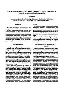
Fig. 1. Number of Tb measurements per bin of incidence angle and distance to the satellite track.

To retrieve SM from SMOS Tb ’s using NNs, one would like to use brightness temperatures with the more straightforward physical interpretation, i.e., in the Earth polarization reference frame. In addition, as a NN should have as input a vector of constant length, it is needed to work with fixed angle bins. Therefore, we have used the Level 3 Brightness Temperature (L3TB) from the CATDS (Centre Aval de Traitement des Données SMOS). The L3TB product [30] is a daily global brightness temperature dataset in a 0.25◦ EASE grid [31] obtained from the L1B product [32]. It includes all the Tb ’s acquired a given day, transformed to the ground polarization reference frame (horizontal, H, and vertical, V, polarization), and averaged within 5◦ -width incidence angle bins. The center of the first angle bin is 2.5◦ . Ascending and descending orbits are processed separately. As the satellite progresses, any given location on the Earth’s surface is “seen” a number of times at different incidence angles depending on the location with respect to the satellite subtrack : the further away, the fewer the angular acquisitions [2]. Fig. 1 show the number of Tb ’s measurements (in H polarization) as a function of the incidence angle and the distance to the satellite subtrack (parameter Xswath) for a subset of L3TB data. Along track, a wide range of angles is obtained (0 to 60◦ ). On the opposite, the only angle range that it is accessible all across the swath is from 40◦ to 45◦ . The data base constructed for this project also contains information from the CATDS L3 UDP (User Data Product) [30], such as the SM obtained by the SMOS operational algorithm (hereafter SMOS L3SM), and the probability of having a Radio Frequency Interference (RFI) at a given position (parameter RFI_Prob).

3

and 09:30 for the descending overpass. ASCAT uses fan-beam antennas that covers two 550-km swaths which are separated from the satellite ground track by about ∼ 336 km. ASCAT measures the backscattered radiation at incidence angles from 25◦ to 65◦ . Passive and active microwaves have different sensitivity to SM, vegetation and roughness. In the case of SMOS and ASCAT, the observing frequency is also different. Thus, ASCAT data is a potentially useful data set to complement SMOS in the framework of NN inversions. However, in order to use ASCAT as input to the NNs, a pre-processing step is necessary to interpolate the backscatter coefficients to the single constant incidence angle. The adopted pre-processing scheme is inspired from the processing chain of the ERS and ASCAT SM products [34], [35]. The reference incidence angle has been chosen to be 40◦ as it is in the middle of the observed incidence angle range [34]. The relationship between backscatter and incidence angle is linear over a large range of angles, therefore the angle interpolation has been done using a linear regression. The time window used to compute the regression has to be large enough to ensure the robustness of the regression, while ensuring that the surface conditions other than SM (in particular the vegetation, which affects the slope) remain nearly constant. As a good compromise, the time window has been chosen to be seven days ending the day one wants to estimate the backscattering coefficient for an incidence angle (θ) of 40◦ (hereafter σ40 ). The slope of the line fitted to the points is determined in the data of this window. In general, the fitted line does not goes through the backscattering coefficient measured for the time t of interest (which has been acquired at a variable angle from 25◦ to 65◦ ). Therefore, a line with the same slope but containing the measurement at time t is computed. This is the line used to estimate σ40 . In summary, the seven-day window is used to compute the slope of the σ(θ) function but the actual line used to compute σ40 is shifted to take into account the backscattering at time t, which depends mainly on the SM content. For many grid points the backscatter coefficient can been measured several times per day at different incidence angles, both in ascending and descending overpasses. A σ40 is computed from each σ value. Finally, the different values are averaged to obtain a daily estimation of σ40 . The more elaborated processing discussed by [34] computes not only the slope but also the curvature of the σ(θ) function. In addition, data from several years are used to reduce the uncertainties in the σ40 estimates by computing averaged values for a particular period of the year. However, Sects. V and VI show that the simpler ASCAT data processing discussed in the current study is enough to show the complementarity of passive and active microwaves to retrieve SM.

B. ASCAT data

C. ECMWF models

The Advanced Scatterometter (ASCAT) is a real aperture radar operating at 5.255 GHz (C-band) onboard EUMETSAT’s Meteorological Operational (MetOp) satellite [33]. MetOp is in a sun-synchronous orbit, with equator crossing times of approximately 21:30 local time for the ascending overpass

The ECMWF products used in this work are operational Integrated Forecasting System (IFS) models with the “Hydrology-improved Tiled ECMWF Scheme for Surface Exchanges over Land” (H-TESSEL) [36]. A significant improvement of H-TESSEL took place in November 9th, 2010


with the addition of: (i) a simplified Extended Kalman Filter for the global operational soil moisture analysis [37], (ii) a new snow analysis based on NESDIS snow cover data at 4 km resolution [38] and, (iii) a monthly varying climatology of leaf area index (LAI) based on MODIS data [39]. Therefore, in this study only data from November 9th, 2010 have been used. The original ECMWF IFS products used in this study have a native resolution of ∼ 25 km [40] similar to that of the CATDS grid. They have been re-sampled to the CATDS EASE grid and temporally interpolated to the time of the SMOS acquisitions for ascending and descending orbits (the IFS products have a temporal sampling of 3 hours). We will use the volumetric moisture content in the first layer (0-7 cm depth, hereafter ECMWF SML1 ) of these models as reference or target SM to train the neural networks. In addition, we have used the snow depth and the soil temperature in the first layer to filter out regions with snow or frozen soils. D. MODIS NDVI The SMOS signal is affected by the vegetation water content. In addition, the presence and amount of vegetation is correlated with SM in many ecosystems. Therefore, a vegetation index could improve the SM retrieval, as it has been found in previous works using other satellite observations and a similar methodology [22], [41]. Here, the MODIS Normalized Difference Vegetation Index (NDVI) product MYD13C1 has been used. The MODIS NDVI product contains atmospherically corrected bi-directional surface reflectances masked for water, clouds, and cloud shadows. Global MYD13C1 data are cloud-free spatial composites of the gridded 16-day 1-kilometer MYD13A2, and are provided as a level-3 product projected on a 0.05◦ geographic Climate Modeling Grid (CMG). Cloud-free global coverage is achieved by replacing clouds with the historical MODIS time series climatology record. A zero-order spatial interpolation of the 0.05◦ MODIS grid to the 0.25◦ CATDS grid has been done. In addition, the 16 days MODIS NDVI value for a given grid point is assigned to that point for the previous 8 days and the following 7 days, without any temporal interpolation. This approach presents the advantage of giving a rough estimate of the vegetation characteristics without imposing strong constrains for instance in an operational context. It will be seen in the following that the introduction of such information actually improves significantly the SM retrieval (Sect. V). E. Wetlands The emissivity of water being typically half of that of dry soil, the brightness temperatures measured by SMOS over water bodies are significantly lower to those measured over soil, even with a high SM content. Big water bodies are filtered using land-water masks. The problem is dealing with inundated areas. If the SMOS pixel is completely covered by free water, the point is easily filtered out using Tb thresholds (see Sect. III-A). For the pixels partially inundated, the situation is more complex. Therefore, in order to have a clean dataset to

4

train the NNs, it is pertinent to introduce an information on wetlands extension on the data base. There are several wetland extension datasets such as the NASA JPL Wetland Extent database [42], the Global Lakes and Wetlands Database (GLWD) [43] and the Global Inundation Extent from Multi-Satellites (GIEMS) dataset [44]. The last two ones have been extensively validated at global scale [45], [46] but the GLWD is a static dataset without temporal variation estimations. Therefore, we have used the GIEMS monthly averages of wetland extensions. F. Texture Soil texture is a fundamental information when dealing with SM as, for instance, the emissivity of a sand or clay soil with the same volumetric SM will be very different (e.g. [47]). This is a consequence of the soil micro-physics as even if the total volumetric soil moisture is the same, there would be many more free water molecules in a sandy soil that will absorb the Earth thermal radiation, reducing the emissivity and the observed Tb ’s. Therefore, giving a texture information to the NN can be important in particular to achieve good retrievals for intermediate values of SM, as those values can be easily measured in soils with a variety of textures. Therefore, the sand and clay fractions from the ECOCLIMAP [48] soil texture maps has been added to the database. This is the same texture information that is used by the SMOS L2 and L3 algorithms [3], [30]. III. DATA ANALYSIS A. Time period and data filtering The data sets presented in Sect. II have been compiled from Nov 9th, 2010 (ECMWF models with improved surface physics, see above) to December 31st, 2012. From this data set we have extracted a subset to perform a sensitivity analysis and the training of the neural networks. The subset samples one full year from two from April 1st, 2011 to March 31st, 2012 to capture the year cycle. During this period, one day over four is kept for the analysis. For each selected day, the subset only contains one grid point every two in latitude and longitude, reducing the total number of points by a factor of 4. Grid cells with a latitude higher than 75◦ or lower than -60◦ or corresponding to water bodies are excluded. Points with frozen soil (soil temperature in the first layer of ECMWF models lower than a threshold of 274 K) or covered by snow (as predicted by ECMWF models) at a given time are also filtered out. The data subset does not include points for which the monthly average wetland fraction is higher than 10%. Regarding the SMOS data, grid cells with a cumulative probability of the presence of RFI higher than 20% or with Tb ’s lower than 50 K or higher than 400 K are filtered out. Finally grid cells corresponding to sites of the USDA-NRCS SCAN network (USA) are also removed from this subset as these sites will be used to perform independent a posteriori tests of the NN retrieval performance (Sect. VI-D). The distribution of SM in the filtered subset is relatively uniform from 0 to ∼ 0.5 m3 /m3 except for the values close to zero. In contrast there is a small number of points with very


5

high SM values from 0.53 to 0.8 m3 /m3 that correspond to peat soils in the arctic regions during northern summer. Those organic soils with SM values of 0.53-0.8 m3 /m3 can de facto be considered as inundated wetlands and the number of these points is less than 1% of the total number of points. Therefore they have been filtered out. The total number of points in the training subset having simultaneously well defined SMOS Tb ’s for incidence angles from 0 to 60◦ , ASCAT σ40 , MODIS NDVI and ECMWF SM1 is ∼ 105 . This number increases by a factor of 3.4 if only SMOS incidence angles from 25◦ to 60◦ are requested as the swath that can be used is wider (Fig. 1). B. Sensitivity to soil moisture In order to better understand the sensitivity of SMOS Tb ’s and other observables to SM, the filtered data subset has been used to compute Pearson correlations coefficients (R) of those observables with respect to ECMWF SM1 . Fig. 2 and Table I show the results. 1) SMOS brightness temperatures: The correlation of SMOS Tb ’s and ECMWF SM1 is globally low both for H and V polarization (blue and red circles, respectively). The correlation increases (in absolute value) for V polarization for increasing incidence angles up to |R|=0.61. Fig. 2 also shows the correlations of other quantities derived from SMOS Tb ’s such as the Tb ’s divided by the soil temperature of the first layer of ECMWF model predictions (blue and red crosses for H and V polarizations, respectively), which are an approximation to the soil emissivity. Nevertheless, the correlation with SM is very close to that of the Tb ’s. The correlation of the normalized polarization difference ((TbH − TbV )/(TbH + TbV ), black diamonds) shows a positive correlation with SM but the absolute values are not higher than those obtained for the Tb ’s alone. The relatively low correlation coefficients discussed above imply that a careful selection of the best set of SMOS Tb ’s is needed to ensure a good retrieval using neural networks. 2) Other physical magnitudes: In addition to SMOS Tb ’s, the correlation of other physical magnitudes with respect to ECMWF SM1 are shown in Table I. The correlation of the soil temperature and the soil sand and clay fractions with ECMWF SM1 is lower than 0.5. The clay fraction is positively correlated with SM because water molecules are captured within the clay. The sand fraction is negatively correlated with the SM content in the first few centimeters of soil (where the thermal emission from the Earth detected by SMOS comes from) because sand favors infiltration. In contrast, the correlation of the daily estimate of ASCAT σ40 and SM is 0.62 and that of MODIS NDVI with SM is 0.80. This high value is partly due to the high seasonal patterns present both in NDVI and SM in some regions of the globe, as shown for instance by [41]. 3) Local normalization of SMOS Tb ’s: It is possible to preprocess SMOS Tb ’s to compute a local index (hereafter index I1 ) by normalizing from 0 to 1 the brightness temperature for each polarization and incidence angle. First, the maximum (Tbmax ) and minimum (Tbmin ) of the Tb ’s in the time series

Fig. 2. Correlation R of H and V brightness temperatures (circles), brightness temperatures divided by the soil temperature (crosses), normalized indexes I1 (triangles) and I2 (squares) with respect to ECMWF SM1 . Blue symbols correspond to H polarization and red to V polarization. Black diamonds give the correlation for the normalized polarization ratio (see Sect. III.) TABLE I C ORRELATION R OF DIFFERENT OBSERVABLES AND ECMWF SM1 .

Obs

Ts

NDVI

sand

clay

σ40

I2σ40

R

-0.17

0.80

-0.33

0.41

0.62

0.87

for a given grid point (i, j) are computed. Then, at a time t, the index I1 is computed as follows: I1 (t, i, j) =

Tb (t, i, j) − Tbmin (i, j) Tbmax (i, j) − Tbmin (i, j)

(1)

This computation is not a trivial normalization of the brightness temperatures globally because it is done independently for each grid point. Fig. 2 shows the correlation of the index I1 with respect to ECMWF SM1 for each incidence angle (blue and red triangles for H and V polarization, respectively). In contrast to the original Tb ’s, the correlation of I1 index with SM is almost independent of the incidence angle with a value of ∼ −0.4. The index I1 can be used to define a new index I2 using the SM values at each grid point (i, j) at the time when Tb reaches max min its minimum SM Tb (i, j) and maximum SM Tb (i, j) as follows: I2 (t, i, j)

min

= SM Tb

+[SM

(i, j) +

Tbmax

min

(i, j) − SM Tb

(i, j)] ×

×I1 (t, i, j)

As I1 , the index I2 is computed for each incidence angle bin and polarization at the time t of the SMOS acquisition. The information content of index I2 is very strong as it contains a local information on the dynamic ranges of both the measured Tb ’s and the model SM. Fig. 2 shows the


correlation R of the index I2 with respect to ECMWF SM1 for each incidence angle (blue and red squares for H and V polarization, respectively). Like index I1 , the correlation of index I2 with SM is almost independent of the incidence angle. In contrast, correlation increases up to values of 0.900.92. Table I also shows the correlation with ECMWF SM1 of the locally normalized index I2 computed with ASCAT σ40 (I2σ40 ), which is also very high (0.87). The definition of indexes I1 and I2 is inspired by the so called “change detection” approach used for SM retrieval with ERS and ASCAT scatterometer data [49]. However, one should bear in mind that in the current study the indexes I1 and I2 are just local normalizations. In contrast, the ASCAT SM retrieval is not a mere scaling between dry and wet soil conditions as done by index I1 , but also corrects for vegetation effects. In addition, the ASCAT SM retrieval does not use modeled SM data as reference as used for calculating index I2 . Instead, dry and wet reference values are estimated by analyzing several years of data [35]. Nevertheless, as discussed above, these simple normalization indexes can be used to improve the performances of the NN retrieval (see also Sect. V). IV. M ETHOD : NEURAL NETWORKS Multilayer feedforward neural networks are universal approximators [50] and a very efficient method to find a function linking a set of input data to SM. In particular, the NN approach can exploit the synergy of different instruments due to its truly multivariate nature and its non-linear capacities [51]. It has been shown that the NN is able to exploit complex interactions among the satellite data so that combining a priori the satellite information into the retrieval scheme gives better results than a posteriori combination of individually retrieved products [21]. The feedforward network used in this work has two layers. Many tests were done to determine the optimal architecture, the transfer functions and the minimization algorithms. Above 5-7 neurons in the hidden layer (depending on the dimension of the input vector) the results do not improve anymore and remain constant up to 20 neurons. Using a NN with three layers (two hidden layers) does not improve the results. This is in agreement with Cybenko [52], who showed that a network with a single layer of sigmoid functions can approximate any continuous function. Using a logarithmic-sigmoid function or an hyperbolic tangent sigmoid function (tansig) gives results in perfect agreement. Several minimization algorithms were tested, finding no differences except in computing time, therefore the Levenberg-Marquard algorithm was preferred. The low sensitivity of the results to those parameters is due to the large statistics in the training database, which contains more than 3 105 vectors. Therefore, the results shown in the following have been obtained with 10 nodes or neurons in the hidden layer and with tansig transfer functions. The second layer is composed of a single node with a linear function. For each neuron in the first layer, the input vector (including a unity element, the bias) is multiplied by a vector of weights using a scalar product. The activation functions associated to each neuron are applied to those scalars. The operation is repeated

6

for the second layer. The vector containing the outputs of the first layer of neurons plus a unity element is again multiplied by a vector of weights and the linear combination is used as the input of the neuron of the second layer constituted of a linear function. Therefore, for an input vector of 8 elements, for instance, a neural network with the former structure will have a total of (8+1)×10+(10+1)×1 = 101 free parameters corresponding to 10 weight vectors of 9 elements and 1 weight vector of 11 elements. For each input vector containing a combination of SMOS Tb ’s, ASCAT σ40 , MODIS NDVI and other data, there is an associated target containing a ECMWF SM1 value. The output of the NN is compared to the target and the weights are adjusted by minimizing a cost function (Mean Squared Error). The minimization has been done by gradient backpropagation with the Levenberg-Marquard algorithm (using the Matlab Neural Network library). The input and the targets have been normalized to fall in the range [-1, 1], as this optimizes the training of the NN. Data in the period from January 1st, 2012 to December 31st, 2012 have been selected for the training (∼ 3 105 vectors). This data subset has been decomposed randomly in 60 % actually used for the training, 20 % for validation and 20 % for test purposes such as to compute the global correlation of NN outputs with the reference SM (Tables II and III). The validation dataset is used to detect signs of overlearning during the minimization (learning). This occurs when the correlation of retrieved SM and target SM improves for the training dataset but the performances start to degrade on the validation dataset. Actually, no signs of overlearning have been detected as the training data base is composed of a large number of statistically significant data. The minimization has been stopped after 30-50 iterations once the cost function has approached asymptotically a minimum. The effect of the weight initialization on the minimization results has been tested, finding that the effect is negligible. Once the training is done, more independent tests have been performed using data from a period that has not been used for the NN training (November 2010 to December 2011), or for locations of in situ stations, from November 2010 to December 2012, since as mentioned in Sect. III-A data from these locations have been removed from the training dataset. V. R ESULTS A. Using SMOS Tb ’s as input 1) Selection of SMOS Tb ’s: As discussed in Sect. III, an appropriate selection of the incidence angles of the SMOS observations is necessary to ensure the best SM retrieval in a fraction of the swath as large as possible. Table II shows a comparison of the SM produced by several NNs applied to ascending orbits data of the test subset (Jan 2012 - Dec 2012) with respect to ECMWF SM1 using three different metrics: the correlation coefficient (R), the root mean squared difference or “error” (RMSE), and the mean absolute difference or “error” (MAE). The retrieval is better using only H polarization than using only V polarization (see for instance results for NN inversions with 7 Tb ’s in H polarization in the


TABLE II E FFECT OF DIFFERENT COMBINATIONS OF SMOS Tb ’ S ON NEURAL NETWORKS RETRIEVALS APPLIED TO ASCENDING ORBITS DATA OF THE TEST SUBSET (JAN 2012 - D EC 2012). T HREE DIFFERENT METRICS ARE GIVEN TO COMPARE THE SM RETRIEVED BY THE NEURAL NETWORK TOR THE EMCWF SM: CORRELATION COEFFICIENT (R), ROOT MEAN SQUARED DIFFERENCE OR ERROR (RMSE), AND MEAN ABSOLUTE DIFFERENCE OR ERROR (MAE).

Input data

R

RMSE

MAE

Using only SMOS brightness temperatures 7Tb V 25-60 7Tb H 25-60 8Tb HV 25-45 12Tb HV 20-50 14Tb HV 25-60 14Tb HV 25-60, 7(V-H)/(H+V) 16Tb HV 20-60

0.68 0.71 0.74 0.76 0.80 0.80 0.79

0.117 0.113 0.104 0.105 0.093 0.093 0.097

0.093 0.091 0.082 0.081 0.072 0.072 0.075

Using soil temperature and texture 14Tb, T 14Tb, tex 14Tb,T,tex

0.83 0.84 0.86

0.086 0.084 0.079

0.066 0.065 0.060

0.078 0.071 0.069

0.059 0.054 0.052

0.085 0.073 0.066

0.071 0.056 0.050

Using NDVI 14Tb,NDVI 14Tb,NDVI,tex 14Tb,NDVI,tex,T

0.87 0.89 0.90 Using ASCAT

14Tb,σ40 14Tb,σ40 ,NDVI 14Tb,σ40 ,NDVI,tex

0.84 0.88 0.91

Using local information on extreme Tb’s 14Tb,14I1 14Tb,14I1 ,NDVI 14Tb,14I1 ,NDVI,tex

0.83 0.88 0.90

0.088 0.075 0.067

0.067 0.057 0.050

angle range from 25 to 60◦ “7Tb H 25-60” and the results for the equivalent model with Tb ’s in V polarization “7Tb V 25-60”). Using a combination of H and V Tb ’s gives better results than using just H or V Tb ’s alone (see for instance the results for NN inversions with 7 Tb ’s in H polarization and 7 Tb ’s in V polarization in the angle range from 25 to 60◦ “14Tb HV 25-60” and the results for the equivalent model with Tb ’s in V polarization “7Tb H 25-60” ), which is logical as the input vector dimension increases by a factor of two. Adding the normalized polarization difference as input (NN 14Tb, 7(H-V)/(H+V)) does not improve the results. Regarding the incidence angle range, Table II shows the results for SM inversions obtained with different sets of input data. The retrieval performance actually improves from using H and V Tb ’s in the angle range from 25 to 45◦ (“8Tb HV 2545”) to 20◦ -50◦ (“12Tb HV 20-50”) and 25◦ -60◦ (“14Tb HV 25-60”). In contrast, using Tb ’s in the 20◦ -60◦ range (16Tbs 20-60) does not improve the quality of the NN SM anymore, while it decreases the width of the swath in which the SM can be obtained (Fig. 1). Therefore, the best set of SMOS Tb ’s to retrieve SM using NNs is composed of 7 Tb ’s for angle bins from 25◦ to 60◦ for both H and V polarizations (a total of 14 Tb ’s).

7

2) Adding additional data as input: a) Soil temperature and texture: In a first approximation the Tb is the product of the soil temperature multiplied by the emissivity. Therefore it is interesting to test the effect of adding the soil temperature as one of the input vector elements for the NN. In addition, the emissivity depends on the dielectric constant of the soil, which depends itself on soil texture (and moisture content, of course). Thus, some information on the soil texture, namely the clay and sand fractions, can potentially improve the SM retrieval. Table II shows the performance of the NN retrieval when adding soil temperature and texture information in addition to 7 SMOS Tb ’s for H and V polarization in the angle range from 25◦ to 60◦ . The addition of temperature or clay and sand fractions improves the correlation of SM retrieved by NN and ECMWF SM by 4% (R). Everything together improve R by 8%. Fig. 3 shows scatter plots of SM retrieved by NN versus ECMWF SM. Interestingly, adding the sand and clay fractions breaks a bi-modality that is present for intermediate SM values in the scatter plot of SM retrieved by a NN with only SMOS Tb ’s as input versus ECMWF SM1 . b) Using a vegetation index: In the presence of vegetation, the Tb ’s measured by SMOS will also depend on the vegetation opacity which attenuates soil radiation and depolarizes the soil signal. Therefore, some information on the vegetation estate is a potential valuable input for the NN. On the other hand, as discussed in Sect. III, the correlation of MODIS NDVI (with only two reference dates per month) and SM is actually very high (R ∼ 0.8), in good agreement with previous studies using other datasets at a monthly scale [22], [24], [41]. This correlation comes from the global close relationship of SM and vegetation at a seasonal scale length, but of course one cannot retrieve accurately the highly changing dynamics of surface SM (at a time scale of a few hours) using just NDVI. In contrast, NDVI helps significantly the retrieval of SM by NN, providing a good “seasonal first guess” while SMOS Tb ’s are instantaneous estimations of the SM content. Table II shows that NDVI actually improves the NN retrieval by 8% (model “14Tb’s, NDVI ”). While the retrieval improves by 11% when adding also soil texture and temperature information (model “14Tb, NDVI, tex, T”), reaching a significantly high correlation of R = 0.9. c) Effect of adding active microwaves: NN retrievals combining active and passive microwave observations have been tested using ASCAT and SMOS data. Using jointly SMOS and ASCAT for SM retrieval at a daily scale is nontrivial since SMOS and ASCAT do not observe the same point at the same time (Sect. II) and SM can change rapidly at the scale of hours. In the current study, the ASCAT active microwave information has been introduced as a daily averaged value, which could damp the sensitivity to SM variations. In addition this value will be compared to ECMWF SM1 estimations interpolated at the time of the SMOS acquisitions. Developing an optimized multi-sensor retrieval is out of the scope of this study, which is mainly devoted to SMOS. However, this relatively simple ASCAT data processing is enough to show that adding active microwaves to the retrieval can improve significantly the results (see Sect. VI-B). Table


8

Fig. 3. SM computed by applying the trained NN to ascending orbits data of the test subset (Jan 2012 - Dec 2012) versus ECMWF SM1 . From top to bottom and from left to right, the scatter plots correspond to NN’s with the following input data: “14Tbs”, “14Tbs, T, tex”, “14Tbs, σ40 , tex, NDVI”, and “14I2 , I2σ40 ” (see Sect. V for a detailed description of those NN retrievals). The black dashed line is the 1:1 line and the black solid line is the regression line. The linear regression equation is given in the bottom of each panel.

II shows the results of SM retrievals using SMOS + ASCAT data. Adding ASCAT improves the SM retrieval by 5% (R). Adding NDVI and soil clay and sand fractions increase R up to 0.91. In this case, adding the soil temperature to the input vector does not improve the performance of the retrieval [53]. d) Using local information on the Tb ’s dynamic range: Table II shows the results of NN retrievals using index I1 . Adding this index to the input vector increases the correlation of NN SM and ECMWF SM1 from R = 0.80 (model “14Tb’s”) to R = 0.83 (model “14Tb’s, I1 ”). Adding the vegetation index the correlation increases to R = 0.88. Adding the soil texture information the correlation increases to R = 0.90, which equals the highest value obtained without I1 . In this case, adding the soil temperature to the input vector does not add any information. The advantages of a retrieval “14Tb’s,I1 , NDVI, tex” with respect to “14Tb’s, NDVI, tex, T” is that it only needs two remote sensing data sets (daily SMOS data and a NDVI estimation every 15 days) and a static texture information. Therefore, once the NN is trained, using model “14Tb, I1 , NDVI, tex”, the SM can be retrieved without ECMWF data. B. Using local information on the Tb ’s and SM dynamic range As discussed in Sect. III, local information on the Tb ’s and SM dynamic range can be used to define the index I2 , which becomes the physical magnitude that shows the highest correlation with ECMWF SM1 (Fig. 2). Of course, this is

TABLE III E FFECT OF DIFFERENT COMBINATIONS OF SMOS INDEX I2 WHEN APPLYING THE TRAINED NN S TO ASCENDING ORBITS DATA OF THE TEST SUBSET (JAN 2012-D EC 2012).

Input data

R

RMSE

MAE

Using local information on extreme Tb’s & SM 2I2 HV40-45 4I2 HV35-45 6I2 HV30-45 8I2 HV25-45 10I2 HV25-50 14I2 HV25-60

0.91 0.91 0.92 0.93 0.93 0.93

0.064 0.064 0.060 0.059 0.059 0.058

0.046 0.046 0.043 0.042 0.042 0.042

Using additional information 14I2 ,I2σ40 14I2 ,I2σ40 ,NDVI 8I2 ,I2σ40 8I2 ,NDVI 8I2 ,NDVI,I2σ40

0.94 0.94 0.94 0.94 0.94

0.055 0.053 0.055 0.055 0.053

0.040 0.038 0.040 0.039 0.038

logical as in this case the NN gets as input some information on the SM magnitude that should be retrieved. Since the linear correlations of I2 and SM are very high, it is likely that using I2 the NN does not need as many input elements as the NN using Tb ’s as input. Actually, even using only one angle bin for the two polarizations (“2I2 HV40-45”), the


correlation coefficient R obtained applying the trained NN to ascending orbits data of the test subset (Jan 2012 - Dec 2012) is already higher than 0.9 (Table III). In addition, such retrieval methodology would allow to retrieve SM for the whole SMOS swath. Correlation increases when adding more I2 indexes for other angle bins up to four angle bins in the range 25-45◦ and two polarizations (“8I2 HV25-45” input). Using more angle bins reduces the RMSE without an increase of R. Table III shows the result for two polarizations and 7 angle bins –14I2 – , which is the equivalent configuration to that giving the best results when using Tb ’s). Using 8I2 and NDVI the retrieval still improves by ∼ 1%. The same score (R=0.94) is also obtained with “14I2 ,I2σ40 ”. When using index I2 , adding the soil temperature and even the soil texture to the input vector does not add any information with respect to the previous models. This is because, the I2 index contains implicitly this information from the local SM values for the extreme Tb ’s. Ideally, computing local extreme Tb ’s and the associated SM values should be done in a period as long as possible to have robust results. In the present study the extreme values have been computed using 2.5 years of data. The effect of using a shorter period has also been tested. When computing the extreme values using only 1 year of data, the global correlation obtained for a given NN configuration decreases by ∼ 2%. The advantage of using I2 is that it allows to perform good retrievals even with a small number of observables given as input to the NN and that it gives the best results in terms of quality metrics with respect to the reference SM dataset. The disadvantage is that potential errors in the local SM time series extreme values used to compute index I2 will be easily replicated in the NN retrieval. In contrast, when not using any SM information as input to the NN, the non-linear regression done during the NN training makes the NN less sensible to outliers in the reference SM dataset [23]. VI. D ISCUSSION A. Reference NN retrievals: maps Five of the best NN models have been selected to perform further evaluation of different SM retrievals using NNs. Those retrievals are shown in Table IV. The retrieval NNSM1 uses as input similar information to that used by the SMOS L3 operational algorithm: SMOS Tb ’s, soil texture and temperature and a vegetation index (NDVI for NNSM1 and LAI for SMOS L3). Retrieval NNSM2 also uses the local normalized Tb ’s (I1 ) in addition to SMOS Tb ’s and NDVI. Retrieval NNSM3 also uses ASCAT data as input. Finally, retrievals NNSM4 and NNSM5 use the change detection approach with SMOS I2 indexes and NDVI (NNSM4 ) or I2σ40 (NNSM5 ). In addition, the best retrieval using only SMOS data as input (NNSM6 ) has also been selected in order to compare its performances with those using the multi-sensor approach. The Level 3 CATDS SMOS products are divided in ascending (equator overpass at 6 am) and descending (6 pm) half-orbits. The reason is that sources of radio-frequency interference (RFI) are often directional and they affect differently morning and evening overpasses. In addition, the evaluation of SMOS products against in situ measurements has shown

9

TABLE IV R ESULTS OBTAINED TRAINING THE REFERENCE NN MODELS ON DESCENDING ORBITS DATA AND APPLYING THE TRAINED NN S TO THE TEST SUBSET (JAN 2012 - D EC 2012).

NN SM

input data

R

RMSE

MAE

NNSM1 NNSM2 NNSM3 NNSM4 NNSM5 NNSM6

14Tb, NDVI, tex, T 14Tb, 14I1 , NDVI.tex 14Tb, NDVI, tex, σ40 8I2 , NDVI 14I2 , I2σ40 14Tb, 14I1

0.91 0.92 0.92 0.95 0.95 0.83

0.067 0.065 0.065 0.052 0.053 0.086

0.050 0.048 0.048 0.037 0.037 0.066

different results for morning and evening overpasses (see also Sect. VI-D and references therein). Therefore, in the current study, data from ascending and descending orbits are also processed independently. The reference NN retrievals have been applied to SMOS data from descending orbits instead of data from ascending orbits as those presented in Tables II and III. The results are shown in Table IV. The NN retrieval quality is comparable (within 1%) to that using ascending orbits. Fig. 4 shows an example of the retrieval NNSM2 for ascending and descending orbits on August 22, 2011 and the corresponding ECMWF SM1 . In addition, the lower panels of Fig. 4 show the monthly average of SM obtained with the retrieval NNSM5 for July 2010 and the corresponding average of ECMWF SM1 . The NN retrievals reproduce the main spatial structures of the ECMWF SM1 dataset. The most significant differences in this example are the drier soil predicted by the NN retrieval in western USA, central Asia and Australia. In addition, the NN retrieval predict somewhat wetter soil in the Sahara desert borders. From the input-data/SM relationship learned globally and over a long time period during the training phase, the NN gives the most likely SM value for a given set of input data [54]. Even if the NN has been trained with ECMWF SM1 , the NN output over a given region at a given time does not necessarily equals the ECMWF SM1 value because the retrieval is driven by the remotely sensed data. In the case shown in Fig. 4, taking into account the global input-data/SM relationship learned by the NN, the ECMWF SM1 values in the western USA, central Asia, Australia and the Sahara-border are not the most likely SM values. At least in the USA, the values predicted by the NNSM retrieval can actually be a statistical correction of ECMWF estimates, as other studies have already shown that ECMWF models are on average too wet in the west of the USA [40], [55]. B. Temporal correlation In order to get further insight on the ability of the neural network with different input data to capture the temporal and spacial variability of the reference ECMWF SM product, it is pertinent to compute temporal (Rtemp ) and spatial correlations (Rspa ) of the NN products with respect to the SM used as reference. This approach has already been used in previous studies [24].


10

Fig. 4. Upper and middle panels show the NNSM2 retrieval for August 22, 2011 for ascending (left upper panel) and descending orbits (left middle panel) and their corresponding ECMWF SM1 estimates (right panels). The lower panel shows the monthly average for July 2010 computed with NNSM5 retrieval applied to ascending orbits (left) and the corresponding ECMWF SM1 (right).

The temporal correlation is defined as the Pearson correlation of the NN SM and ECMWF SM1 time series of each grid point. Rtemp has only been computed if the time series for the whole period of this study contains more than 30 points. Fig. 5 shows maps of Rtemp for the different retrievals. First, there exist regions with negative correlation such as the Sahara region. Fig. 6 shows the variance of the ECMWF SM1 time series for each grid point. There are clear similarities between the variance and the Rtemp maps, showing that regions with negative Rtemp are those where the variance of the local time series is very low. In addition, in this arid region the SM content is also very low. Therefore, the relative uncertainties of the different SM estimations are very high. This makes that when comparing two different SM products over these areas, the correlation is low in absolute value and can even be negative. It is interesting to note that there are significant differences for the different NNSM retrievals that were not obvious in the global correlations shown in Tables II and III. Table V shows the average Rtemp computed for each of the maps in Fig. 5. Both for retrievals using SMOS Tb ’s or the change detection approach, those with a better ability to capture the temporal dynamics of the ECMWF SM1 data are those that include active microwaves data as input (NNSM3 and NNSM5 , respectively). This is in agreement with previous studies that already pointed out the good performance of active microwave data to capture the soil moisture temporal

variability [24], [56]. However, it is worth-noting that the passive microwaves ability to capture the temporal variability can be similar to those of active microwaves when using the local normalization of SMOS Tb ’s (index I1 ) in addition to the Tb ’s themselves as input to the NN (retrieval NNSM2 , Table. V). Even retrieval NNSM6 , using only SMOS Tb ’s and I1 shows a better ability to capture the temporal variability of SM than retrieval NNSM1 . Both NNSM2 and NNSM3 give an average Rtemp higher than retrieval NNSM4 , which uses the SM change detection approach. Nevertheless, the best Rtemp is obtained when using this approach both with active and passive microwaves as input to the NN (SMNN5). With the exception of retrieval NNSM1 , the multi-sensor retrievals perform better than the best SMOS-only retrieval by 8-17%. C. Spatial correlation In addition to the maps of local temporal correlation, it is interesting to compute time series of global daily correlations, which are sometimes called “spatial” correlations, by computing the Pearson 1-D correlation coefficient comparing the values of two daily SM maps (NN SM and ECMWF SM1 ) for all grid points. One should bear in mind that these values are not the 2D cross-correlation of the two SM maps but in the following, the “spatial” correlation, Rspa , terminology will be used for simplicity. Fig. 7 shows the time series of spatial or daily correlation of retrievals NNSM1 and NNSM5 with respect to ECMWF


11

Fig. 6. Variance of the reference ECMWF SM1 time series in logarithmic scale. TABLE V T EMPORAL CORRELATION OF NN AND ECMWF SM AVERAGED OVER ALL THE GLOBE POINTS WITH MORE THAN 30 MEASUREMENTS FOR EACH OF THE REFERENCE MODELS

Retrieval

mean Rtemp A orbits

mean Rtemp D orbits


0.47 0.54 0.55 0.52 0.58 0.48

0.49 0.57 0.56 0.52 0.57 0.53

snow pack filter keeps more points in this months coming from northern high latitude regions. This imply that NN SM predictions are less consistent with ECMWF SM1 in these regions (the maps of Rtemp also show lower values in the northern regions). The typical amplitude of the seasonal oscillation in the Rspa time series is ∼ 10% for retrievals NNSM1−3 and ∼ 5% for retrievals NNSM4−5 . The mean values of Rspa are 0.90-0.91 for retrievals NNSM1−3 and 0.94 for retrievals NNSM4−5 . The retrieval NNSM6 , which uses only SMOS data as input, shows an ability to capture the SM spatial variability that is 6-10% lower than that of the multisensor retrievals. All these values are in perfect agreement with the global correlation computed with the test dataset during the training period discussed in Sect. V. In any case, the Rspa time series imply that the NN retrieval is robust as its performances when applied to data not included in the training dataset are comparable to the performances obtained over the training period. Fig. 5. Maps of temporal correlations for models NNSM 1 to 6 (from top to bottom) applied to SMOS ascending orbits.

SM1 . Time series of Rspa for retrievals NNSM2 and NNSM3 are very similar to that of NNSM1 (and NNSM4 very similar to NNSM5 ) and they are not shown in this figure. Table VI gives the mean Rspa for each retrieval as computed from the corresponding time series. The time series of Rspa show a seasonal oscillation, with slightly lower values for the months of northerns summer. This is because the frozen soil and

D. Comparison with in situ measurements A full validation of SMOS L3 SM, ECMWF SM1 and NN SM with respect to in situ measurements for a variety of ecosystems, physical conditions, or regions is beyond the scope of this paper. However, it is interesting to compare the different NN retrievals discussed above to in situ measurements. Therefore, the reference NNSM retrievals, SMOS L3 SM and ECMWF SM1 have been compared to in situ measurements made by the SCAN network of the US Department of Agriculture [57]. This network has already been used to evaluate modeled SM products as well as SM retrievals from remote


Fig. 7. Temporal series of spatial correlation for retrievals NNSM1 (upper panel) and NNSM5 (lower panel) applied to SMOS ascending orbits. TABLE VI S PATIAL CORRELATION OF NN AND ECMWF SM AVERAGED OVER ALL DAYS FOR EACH OF THE REFERENCE MODELS

Retrieval

mean Rspa A orbits

mean Rspa D orbits


0.90 0.91 0.91 0.94 0.94 0.84

0.91 0.91 0.91 0.95 0.95 0.85

sensing data (ASCAT, SMOS,...), including monthly estimates using NNs [24], [40], [55]. The SCAN data have been obtained from the International Soil Moisture Network [58]. Since Lband radiation is emitted by the first few centimeters under the soil surface [59], the SM products have been compared to in situ SM measurements in the 0-5 cm depth range. A total of 188 time series of in situ measurements have been used to evaluate the SM products. The in situ measurements have been compared with the closest CATDS EASE grid point. The different SM products have been compared at the time of SMOS overpasses. The in situ SM is measured every 30 minutes. Thus, the closest measurement in time to the SMOS overpass has been selected. Of course, one should keep in mind that in situ sensors make a local measurement that is not necessarily representative of the spatial resolution of the remote sensors or the numerical weather prediction models (tenths of kilometers). Some reasons of possible discrepancies are the presence of irrigated areas, water bodies or local precipitations within the SMOS synthesized beam footprint. In addition, the topography or soil texture differences will affect the hydrological processes taking place at the scale of tenths of km, making a single point measurement not representative of the remotely sensed area. However, the large number of SCAN sites allows to do a statistical analysis of the results. In order to have as consistent

12

statistics among the different products as possible, for each time series, it hs been used only the times for which all in situ, ECMWF SM1 , SMOS L3 SM and NN SM are available. In addition, a minimum number of 30 days per time series has been required to compute statistics. The computation has been done independently for ascending and descending SMOS orbits in the full period of this study (Nov 2010 - Dec 2012). It is important to remind that, as mentioned in Sect. III, the EASE grid points corresponding to SCAN sites have been voluntarily excluded from the training data base for them to be used as testing data. For each site, the standard deviation of the difference (STDD) of ECMWF SM1 , SMOS L3 SM and NNSM with respect to the in situ measurement has been computed. In addition, the Pearson correlation (R) of those products with respect to the in situ SM and the bias (defined as the mean of the difference time series) have also been computed. Finally, the minimum, maximum, mean and median values of all those metrics have been calculated. The results are summarized in Table VII. The retrieval NNSM1 , which uses as input similar information to that used by the SMOS L3 algorithm, shows a correlation with the in situ measurements similar to that of SMOS L3 SM. Both for ascending and descending SMOS orbits, NNSM1 and SMOS L3 SM give the lowest average correlation with the in situ data (0.52 and 0.45-0.48 for ascending and descending orbits, respectively). The correlation is higher for the SMOSonly retrieval NNSM6 that uses index I1 (0.53-0.55) and it increases to 0.59-0.61 for NNSM retrievals that include active microwaves data and/or a SM change detection approach (I2 ) such as NNSM 2, 4 and 5. Interestingly, the NNSM3 retrieval, which uses locally normalized brightness temperatures (I1 ), also gives R values of the same order, confirming the interest of this approach that does not include any a priori information on SM to capture the temporal variability of the SM time series (see also Sect. VI-B). ECMWF SM1 also shows a correlation with the in situ measurements of 0.59-0.61 both for ascending and descending orbits. Regarding the STDD, the highest values are given by the SMOS L3 SM time series (0.06-0.07) followed by ECMWF SM1 (∼ 0.05). NNSM 1-3 retrievals present a STDD of 0.04-0.05, and those using the change detection approach NNSM 4-5 present a fairly low STDD of (∼ 0.03). Regarding the bias, NNSM retrievals show a positive bias similar to the ECMWF SM1 , which is logical as the NNs have been trained with ECMWF data. In contrast, SMOS L3 SM shows a negative bias. The bias values obtained for ECMWF SM1 and SMOS L3 SM are in agreement with previous SM products evaluation studies over the SCAN sites [40], [55] and other USA watersheds [60], [61]. The correlations obtained at the time of SMOS descending overpasses are clearly lower than those for ascending overpasses for all SMOS-based products (NNSM and SMOS L3SM). This is also in agreement with previous studies, which have interpreted this fact as the possible effect of convective rainfall, which occurs during the day affecting potentially differently the local in situ measurement and the ∼ 40 km remote sensing measurement and decreasing the


correlation for descending overpasses, which take place in the afternoon/evening [62]. However, it is interesting to note that proportionally, the difference in correlation for ascending and descending orbits is lower for NNSM retrievals using the daily σ40 estimation from active microwaves (NNSM 2) and for the retrievals using the change detection approach. In summary, the comparison of the NNSM retrievals to USDA/SCAN in situ measurements shows the good performances of these retrievals. Products NNSM 4 and 5 (using the local extremes of SMOS brightness temperatures and the associated ECMWF SM1 values) give the best statistics of all the SM products discussed in this study (ECMWF SM1 , SMOS L3, NNSM). E. Comparison with previous NN retrievals of SM at global scale The use of NNs to perform a SM retrieval from multiinstrument observations havs already been studied using active microwaves (ERS), passive microwaves (SSM/I), NDVI (AVHRR) and skin temperature (ISCCP) as input data [22]– [24]. The NNs were trained with different surface physics models forced with numerical weather prediction models. In all those studies the NN approach was evaluated with monthly averages while the current paper describes a daily retrieval. Nevertheless, it is interesting to compare some results of the current study to those of previous studies since they use the approach proposed by [22] but with different input datasets. The monthly SM inversion using NNs by [23] and the JULES land surface model show a global correlation R of 0.92. The SM inversion discussed in the current paper is able to capture the variability of ECMWF model SM in daily basis as it shows a global correlation varying from 0.9 to 0.94 depending on the exact input datasets. On the other hand, the spatial and temporal correlations between the retrieved and the reference monthly SM average found in [24] are 0.81-0.90 and 0.54-0.67, respectively. In the current work, the spatial and temporal correlation in between the daily retrieved SM and the reference one has been found to be 0.90-0.95 and 0.47-0.58, respectively (Tables V and VI). Therefore, the values obtained in the current study for the temporal correlation at daily bases are close to those obtained by [24] using monthly averages. Finally, the monthly SM estimation by [24] has also been compared to the in situ measurements from the SCAN network obtaining a temporal correlation of -0.07, much lower than that of other SM products like HTESSEL (0.72). In contrast, the daily NNSM retrievals discussed in the current study show a similar temporal correlation to that of ECMWF/HTESSEL (∼ 0.60, Table VII). The current study using SMOS and previous studies of global SM retrieval using SSM/I [22]–[24] use the same approach (training a NN to link a multi-sensor input dataset to a reference SM from a land surface model). Therefore, the good temporal and spatial correlation between the NNSM retrievals obtained on a daily basis and ECMWF SM1 or in situ measurements confirm the strong sensitivity of SMOS to SM compared to the non-dedicated microwave observations used by those previous studies [22]–[24].

13

VII. S UMMARY AND CONCLUSIONS A methodology to retrieve soil moisture from multiinstrument observations on daily basis has been presented. The approach is based on a feed-forward neural network using SMOS brightness temperatures (passive microwaves at 1.4 GHz), ASCAT backscattering coefficient (active microwaves at 5.3 GHz), MODIS NDVI and ECOCLIMAP soil texture maps. The neural networks have been trained using ECMWF Integrated Forecast System models, which include soil moisture estimations in the 0-7 cm depth range (ECMWF SM1 ). The best compromise to retrieve SM from SMOS Tb ’s over a large fraction of the swath (∼ 670 km) is to use SMOS data in the incidence angle range from 25◦ to 60◦ (in 7 bins of 5◦ width). The global correlation coefficient of the SM retrieved by NN and ECMWF SM1 is ∼ 0.9 for NN retrievals that, in addition to SMOS Tb ’s, use MODIS NDVI, soil texture and one of the following: (i) ASCAT σ40 , (ii) ECMWF soil temperature or (iii) 14 normalized Tb’s computed using the minimum and maximum values of Tb ’s for each incidence angle and polarization at each latitude and longitude grid point. A change detection approach (defining a local normalization of brightness temperatures using the extreme values and the associated SM) has also been discussed. In this case, soil texture or temperature become irrelevant as the information is implicitly contained in the SM values for the extreme Tb ’s. Using only this approach with SMOS Tb ’s and ASCAT backscattering or NDVI, one can obtain a correlation R of 0.94 between the SM retrieved by NN and the reference ECMWF SM used as target for the NN learning phase. In addition, one advantage of the change detection approach is that good results can be obtained using SMOS data for a lower number of incidence angles, allowing a retrieval over a larger swath (and hence a better temporal coverage). It has been shown that the NNs are able to capture the spatial and temporal variability of soil moisture. The temporal variability is better reproduced when using retrievals schemes that include active microwave information or, alternatively, using only passive microwave data that include a local normalization of SMOS brightness temperatures. When compared to in situ measurements, the NNSM retrievals perform well. Actually, the NNSM retrievals that use a local normalization of the SMOS brightness temperatures and the associated extreme SM values give the best results of all the products evaluated in this study (ECMWF SML1, SMOS L3, NN SM). We have discussed different strategies to retrieve SM from SMOS observations using NNs that perform very well. The best model would depend on the particular application of the NN retrieval. For instance, for an operational NN algorithm using ASCAT will require access to ASCAT data in real time and in addition this data has to be preprocessed to estimate the backscattering at 40◦ incidence angle first, which can put strong constrains on an operational algorithm. In addition, requiring both SMOS and ASCAT observations of the same point reduces the coverage to the intersection of the swaths of the instruments of both satellites. In contrast, MODIS NDVI improves significantly the NN retrieval and it is a very soft


14

TABLE VII C OMPARISON WITH in situ MEASUREMENTS . T HE STANDARD DEVIATION OF THE DIFFERENCE (STDD), CORRELATION COEFFICIENT (R) AND BIAS HAS BEEN COMPUTED FOR ALL SCAN SITES WITH MORE THAN 30 COINCIDENT POINTS IN THE FOUR TIME SERIES (NNSM, ECMWF, SMOS L3 AND in situ). U SING THESE METRICS THE MINIMUM , MEAN , MEDIAN AND MAXIMUM VALUES HAVE BEEN COMPUTED . T HE RESULTS ARE DISPLAYED FOR NN S TRAINED ON SMOS ASCENDING AND DESCENDING ORBITS .

STDD

SM product

Min

Mean

Median

R Max

Min

Mean

Bias Median

Max

Min

Mean

Median

Max

0.58 0.67 0.70 0.69 0.69 0.54 0.64 0.57

0.90 0.90 0.89 0.93 0.89 0.87 0.90 0.89

-0.065 -0.081 -0.080 -0.12 -0.13 -0.13 -0.12 -0.24

0.076 0.075 0.067 0.054 0.052 0.092 0.050 -0.021

0.065 0.076 0.059 0.045 0.034 0.092 0.039 -0.015

0.23 0.22 0.22 0.30 0.30 0.21 0.30 0.10

0.47 0.69 0.63 0.69 0.66 0.63 0.66 0.55

0.92 0.95 0.93 0.96 0.95 0.90 0.89 0.94

-0.096 -0.071 -0.074 -0.123 -0.138 -0.079 -0.138 -0.259

0.070 0.071 0.063 0.056 0.057 0.076 0.061 -0.051

0.061 0.065 0.059 0.036 0.041 0.073 0.046 -0.051

0.30 0.31 0.30 0.38 0.39 0.29 0.38 0.13

Ascending orbits NNSM1 NNSM2 NNSM3 NNSM4 NNSM5 NNSM6 ECMWF SM1 SMOS L3

0.018 0.017 0.013 0.006 0.005 0.025 0.012 0.027

0.046 0.049 0.044 0.029 0.027 0.055 0.049 0.060

0.043 0.046 0.041 0.026 0.023 0.056 0.045 0.059

0.086 0.088 0.074 0.066 0.061 0.102 0.116 0.127

NNSM1 NNSM2 NNSM3 NNSM4 NNSM5 NNSM6 ECMWF SM1 SMOS L3

0.019 0.011 0.014 0.004 0.003 0.022 0.011 0.024

0.045 0.046 0.043 0.033 0.032 0.051 0.053 0.068

0.041 0.044 0.038 0.028 0.026 0.050 0.056 0.065

0.097 0.089 0.084 0.094 0.100 0.098 0.129 0.148

-0.15 0.08 0.13 0.12 0.033 0.051 0.075 -0.13

0.52 0.60 0.61 0.61 0.60 0.55 0.59 0.52

Descending orbits -0.12 -0.41 -0.17 -0.22 -0.18 -0.17 0.01 -0.41

constrain to a real time pipeline as only one NDVI every 15 days is used for the NN retrieval. Adding soil texture improves the results by ∼ 3%, but soil texture is a static information that does not make more complex a real time algorithm. Retrieval schemes using local normalization indexes need a few years of data for the indexes to be significant but they are less dependent on external datasets and they allow to retrieve SM over a larger swath because a lower number of incident angles are required. Once trained, NNs are a very efficient method to retrieve SM. For instance, using the data filtering discussed in Sect. III, applying the NN to all SMOS ascending orbits in the data base discussed in this paper (with more than 2 years of data) takes ∼ 150 seconds on a standard desktop computer. This fact opens exciting perspectives for a near-real-time operational product. Training NNs with a numerical weather prediction model ensures that the retrieved SM is consistent with the model. However, the NN SM can correct the model accordingly to the remote sensing observations. Therefore, this approach can be the basis for an efficient satellite data assimilation into numerical weather prediction models [22]. Meteorological offices need satellite data no more than 3 hours after sensing to be able to assimilate the observations in a forecasting system. A near-real-time algorithm using NNs such as those discussed in the current study will be able to retrieve SM fast enough to be assimilated into such a system. ACKNOWLEDGMENT These research has been partly funded by the SMOS+”Neural Networks” ESA ESRIN project under

0.45 0.59 0.56 0.59 0.59 0.53 0.61 0.48

contract 4000105455/12. The authors would like to thank CNES and TOSCA (Terre Océan Surfaces Continentales et Atmosphère) program for funding part of this research work. This research made use of data from the Centre Aval de Traitement des Données SMOS (CATDS), operated for the Centre National d’Etudes Spatiales (CNES, France) by IFREMER (France). We thank A. Al Bitar for providing the MODIS NDVI data interpolated in the CATDS grid.

R EFERENCES [1] S. Mecklenburg, M. Drusch, Y. H. Kerr, J. Font, M. Martin-Neira, S. Delwart, G. Buenadicha, N. Reul, E. Daganzo-Eusebio, R. Oliva, and R. Crapolicchio, “ESA’s Soil Moisture and Ocean Salinity Mission: Mission Performance and Operations,” IEEE Transactions on Geoscience and Remote Sensing, vol. 50, no. 5, pp. 1354–1366, May 2012. [Online]. Available: http://ieeexplore.ieee.org/lpdocs/epic03/wrapper.htm?arnumber=6175118 [2] Y. Kerr, P. Waldteufel, J.-P. Wigneron, S. Delwart, F. Cabot, J. Boutin, M.-J. Escorihuela, J. Font, N. Reul, C. Gruhier, S. Juglea, M. Drinkwater, A. Hahne, M. Martin-Neira, and S. Mecklenburg, “The SMOS mission: New tool for monitoring key elements ofthe global water cycle,” Proceedings of the IEEE, vol. 98, no. 5, pp. 666–687, May 2010. [3] Y. H. Kerr, P. Waldteufel, P. Richaume, J. P. Wigneron, P. Ferrazzoli, A. Mahmoodi, A. Al Bitar, F. Cabot, C. Gruhier, S. E. Juglea, D. Leroux, A. Mialon, and S. Delwart, “The SMOS Soil Moisture Retrieval Algorithm,” IEEE Transactions on Geoscience and Remote Sensing, vol. 50, pp. 1384–1403, May 2012. [4] C. Jiménez, P. Eriksson, and D. Murtagh, “First inversions of observed submillimeter limb sounding radiances by neural networks,” Journal of geophysical research, vol. 108, no. D24, p. 4791, 2003. [5] F. Aires, A. Chedin, N. A. Scott, and W. B. Rossow, “A regularized neural net approach for retrieval of atmospheric and surface temperatures with the iasi instrument,” Journal of Applied Meteorology, vol. 41, no. 2, pp. 144–159, 2002.


[6] A. Niang, L. Gross, S. Thiria, F. Badran, and C. Moulin, “Automatic neural classification of ocean colour reflectance spectra at the top of the atmosphere with introduction of expert knowledge,” Remote Sensing of Environment, vol. 86(2), pp. 257–271, 2003. [7] P. Richaume, F. Badran, M. Crepon, C. Mej´ıa, H. Roquet, and S. Thiria, “Neural network wind retrieval from ERS-1 scatterometer data,” Journal of Geophysical Research, vol. 105(C4), p. 8737–8751, 2000. [8] C. Jiménez, C. Prigent, and F. Aires, “Toward an estimation of global land surface heat fluxes from multisatellite observations,” Journal of Geophysical Research, vol. 114, no. D6, Mar. 2009. [9] F. Aires and C. Prigent, “Toward a new generation of satellite surface products?” Journal of Geophysical Research: Atmospheres (1984–2012), vol. 111, no. D22, 2006. [10] A. Elshorbagy and K. Parasuraman, “On the relevance of using artificial neural networks for estimating soil moisture content,” Journal of Hydrology, vol. 362, no. 1–2, pp. 1 – 18, 2008. [Online]. Available: http://www.sciencedirect.com/science/article/pii/S0022169408004204 [11] C. Notarnicola, M. Angiulli, and F. Posa, “Soil Moisture Retrieval From Remotely Sensed Data: Neural Network Approach Versus Bayesian Method,” Geoscience and Remote Sensing, IEEE Transactions on, vol. 46, no. 2, pp. 547–557, Jan. 2008. [12] S. Paloscia, P. Pampaloni, and S. Pettinato, “A comparison of algorithms for retrieving soil moisture from ENVISAT/ASAR images,” Remote Sensing, 2008. [13] N. Pierdicca, P. Castracane, and L. Pulvirenti, “Inversion of Electromagnetic Models for Bare Soil Parameter Estimation from Multifrequency Polarimetric SAR Data,” Sensors, vol. 8, no. 12, pp. 8181–8200, Dec. 2008. [Online]. Available: http://www.mdpi.com/14248220/8/12/8181/ [14] S.-F. Liu, Y.-A. Liou, W.-J. Wang, J.-P. Wigneron, and J.-B. Lee, “Retrieval of crop biomass and soil moisture from measured 1.4 and 10.65 GHz brightness temperatures,” Geoscience and Remote Sensing, IEEE Transactions on, vol. 40, no. 6, pp. 1260–1268, Jun. 2002. [15] F. Del Frate, P. Ferrazzoli, and G. Schiavon, “Retrieving soil moisture and agricultural variables by microwave radiometry using neural networks,” Remote sensing of environment, vol. 84, no. 2, pp. 174–183, Feb. 2003. [16] S.-S. Chai, J. P. Walker, O. Makarynskyy, M. Kuhn, B. Veenendaal, and G. West, “Use of Soil Moisture Variability in Artificial Neural Network Retrieval of Soil Moisture,” Remote Sensing, vol. 2, no. 1, pp. 166–190, Jan. 2010. [17] S. Paloscia, S. Pettinato, E. Santi, C. Notarnicola, L. Pasolli, and A. Reppucci, “Soil moisture mapping using sentinel-1 images: Algorithm and preliminary validation,” Remote Sensing of Environment, vol. 134, pp. 234–248, 2013. [18] E. Santi, S. Paloscia, S. Pettinato, and G. Fontanelli, “A prototype ann based algorithm for the soil moisture retrieval from l-band in view of the incoming smap mission,” in Microwave Radiometry and Remote Sensing of the Environment (MicroRad), 2014 13th Specialist Meeting on. IEEE, 2014, pp. 5–9. [19] E. Santi, S. Pettinato, S. Paloscia, P. Pampaloni, G. Macelloni, and M. Brogioni, “An algorithm for generating soil moisture and snow depth maps from microwave spaceborne radiometers: Hydroalgo,” Hydrology and Earth System Sciences Discussions, vol. 9, no. 3, pp. 3851–3900, 2012. [20] A. Gruber, S. Paloscia, E. Santi, C. Notarnicola, L. Pasolli, T. Smolander, J. Pulliainen, H. Mittelbach, W. Dorigo, and W. Wagner, “Performance inter-comparison of soil moisture retrieval models for the metop-a ascat instrument,” in Geoscience and Remote Sensing Symposium (IGARSS), 2014 IEEE International. IEEE, 2014, pp. 2455–2458. [21] F. Aires, O. Aznay, C. Prigent, M. Paul, and F. Bernardo, “Synergistic multi-wavelength remote sensing versus a posteriori combination of retrieved products: Application for the retrieval of atmospheric profiles using metop-a,” Journal of Geophysical Research: Atmospheres (1984– 2012), vol. 117, no. D18, 2012. [22] F. Aires, C. Prigent, and W. B. Rossow, “Sensitivity of satellite microwave and infrared observations to soil moisture at a global scale: 2. Global statistical relationships,” Journal of Geophysical Research, vol. 110, no. D11, 2005. [23] C. Jiménez, D. B. Clark, J. Kolassa, F. Aires, and C. Prigent, “A joint analysis of modeled soil moisture fields and satellite observations,” Journal of Geophysical Research: Atmospheres, vol. 118, no. 12, pp. 6771–6782, 2013. [Online]. Available: http://dx.doi.org/10.1002/jgrd.50430 [24] J. Kolassa, F. Aires, J. Polcher, C. Prigent, C. Jimenez, and J. M. Pereira, “Soil moisture retrieval from multi-instrument observations: Information content analysis and retrieval methodology,” Journal of

15

[25]

[26]

[27]

[28]

[29]

[30] [31] [32] [33] [34]

[35]

[36]

[37]

[38]

[39]

[40]

[41]

[42]

[43]

Geophysical Research: Atmospheres, vol. 118, no. 10, pp. 4847–4859, 2013. [Online]. Available: http://dx.doi.org/10.1029/2012JD018150 G. Balsamo, E. Dutra, S. Boussetta, A. Beljaars, P. Viterbo, and B. van den Hurk, “Recent advances in land surface modelling at ecmwf,” in ECMWF/GLASS workshop on Land Surface Modelling, 2010, pp. 9– 12. A. Ammar, S. Labroue, E. Obligis, C. E. Mejia, M. Crepon, and S. Thiria, “Sea Surface Salinity Retrieval for the SMOS Mission Using Neural Networks,” Geoscience and Remote Sensing, IEEE Transactions on, vol. 46, no. 3, pp. 754–764, Apr. 2008. B. Berthelot, F. Cabot, and Y. Kerr, “Estimation of soil moisture from SMOS SEPSBIO simulated dataset using neural network,” in Poster seesion, 7th SMOS Workshop, ESA ESRIN Frascati, Italy October 2931,, 2007. K. D. McMullan, M. Brown, M. Martin-Neira, W. Rits, S. Ekholm, J. Marti, and J. Lemanczyk, “Smos: The payload,” Geoscience and Remote Sensing, IEEE Transactions on, vol. 46, no. 3, pp. 594–605, March 2008. E. Anterrieu and A. Khazaal, “Brightness Temperature Map Reconstruction from Dual-Polarimetric Visibilities in Synthetic Aperture Imaging Radiometry,” IEEE Transactions on Geoscience and Remote Sensing, vol. 46, no. 3, pp. 606–612, Sep. 2008. [Online]. Available: http://ieeexplore.ieee.org/lpdocs/epic03/wrapper.htm?arnumber=4456807 L. Berthon, “SMOS CATDS Level 3 Soil Moisture products,” European Geosciences Union General Assembly 2012, pp. 1–1, Apr. 2012. M. J. Brodzik and K. W. Knowles, “Ease-grid: A versatile set of equalarea projections and grids,” Discrete global grids, 2002. J. Barbosa and M. Zapata, “SMOS Level 1 and Auxiliary Data Products Specifications v5.23,” SO-TN-IDR-GS-0005, pp. 1–498, Feb. 2012. R. V. Gelsthorpe, E. Schied, and J. J. W. Wilson, “Ascat- metop’s advanced scatterometer,” ESA bulletin, vol. 102, pp. 19–27, 2000. W. Wagner, G. Lemoine, M. Borgeaud, and H. Rott, “A study of vegetation cover effects on ers scatterometer data,” Geoscience and Remote Sensing, IEEE Transactions on, vol. 37, no. 2, pp. 938–948, Mar 1999. Z. Bartalis, W. Wagner, V. Naeimi, S. Hasenauer, K. Scipal, H. Bonekamp, J. Figa, and C. Anderson, “Initial soil moisture retrievals from the METOP-A Advanced Scatterometer (ASCAT),” Geophysical Research Letters, vol. 34, no. 2, p. 20401, Oct. 2007. G. Balsamo, A. Beljaars, K. Scipal, P. Viterbo, B. van den Hurk, M. Hirschi, and A. K. Betts, “A revised hydrology for the ECMWF model: Verification from field site to terrestrial water storage and impact in the integrated forecast system,” Journal of hydrometeorology, vol. 10, no. 3, pp. 623–643, 2009. P. de Rosnay, M. Drusch, D. Vasiljevic, G. Balsamo, C. Albergel, and L. Isaksen, “A simplified extended kalman filter for the global operational soil moisture analysis at ecmwf,” Quarterly Journal of the Royal Meteorological Society, 2012. E. Dutra, G. Balsamo, P. Viterbo, P. M. Miranda, A. Beljaars, C. Schär, and K. Elder, “An improved snow scheme for the ecmwf land surface model: description and offline validation,” Journal of Hydrometeorology, vol. 11, no. 4, pp. 899–916, 2010. [Online]. Available: http://journals.ametsoc.org/doi/abs/10.1175/2010JHM1249.1 S. Boussetta, G. Balsamo, A. Beljaars, T. Kral, and L. Jarlan, “Impact of a satellite-derived leaf area index monthly climatology in a global numerical weather prediction model,” International Journal of Remote Sensing, vol. 34, no. 9-10, pp. 3520–3542, 2013. C. Albergel, P. de Rosnay, C. Gruhier, J. Muñoz-Sabater, S. Hasenauer, L. Isaksen, Y. Kerr, and W. Wagner, “Evaluation of remotely sensed and modelled soil moisture products using global ground-based in situ observations,” Remote Sensing of Environment, vol. 118, pp. 215–226, 2012. C. Prigent, F. Aires, W. B. Rossow, and A. Robock, “Sensitivity of satellite microwave and infrared observations to soil moisture at a global scale: Relationship of satellite observations to in situ soil moisture measurements,” Journal of Geophysical Research: Atmospheres, vol. 110, no. D, p. 7110, Apr. 2005. K. C. McDonald, B. Chapman, E. Podest, R. Schroeder, S. Flores, K. Willacy, M. Moghaddam, J. Whitcomb, L. Hess, and J. S. Kimball, “Monitoring inundated wetlands ecosystems with satellite microwave remote sensing in support of earth system science research,” in Conference Paper 34th International Symposium on Remote Sensing of Environment–The GEOSS Era: Towards Operational Environmental Monitoring, 4p, 2011. B. Lehner and P. Döll, “Development and validation of a global database of lakes, reservoirs and wetlands,” Journal of Hydrology, vol. 296, no. 1, pp. 1–22, 2004.


[44] C. Prigent, F. Papa, F. aires, W. B. Rossow, and E. Matthews, “Global inundation dynamics inferred from multiple satellite observations, 19932000,” Journal of Geophysical Research: Atmospheres, vol. 112, no. D, p. 12107, Jun. 2007. [45] F. Papa, C. Prigent, F. aires, C. Jimenez, W. B. Rossow, and E. Matthews, “Interannual variability of surface water extent at the global scale, 1993–2004,” Journal of Geophysical Research, vol. 115, no. D12, Jun. 2010. [Online]. Available: http://www.agu.org/pubs/crossref/2010/2009JD012674.shtml [46] E. Fluet-Chouinard, B. Lehner, L.-M. Rebelo, F. Papa, and S. K. Hamilton, “Development of a global inundation map at high spatial resolution from topographic downscaling of coarse-scale remote sensing data,” Remote Sensing of Environment, vol. 158, pp. 348–361, 2015. [47] M. Dobson, F. Ulaby, M. Hallikainen, and M. El-Rayes, “Microwave Dielectric Behavior of Wet Soil-Part II: Dielectric Mixing Models,” IEEE Transactions on Geoscience and Remote Sensing, vol. 23, pp. 35–46, Jan. 1985. [48] V. Masson, J.-L. Champeaux, F. Chauvin, C. Meriguet, and R. Lacaze, “A global database of land surface parameters at 1-km resolution in meteorological and climate models,” Journal of climate, vol. 16, no. 9, pp. 1261–1282, 2003. [49] W. Wagner, G. Lemoine, and H. Rott, “A Method for Estimating Soil Moisture from ERS Scatterometer and Soil Data,” Remote sensing of environment, vol. 70, no. 2, pp. 191–207, Oct. 1999. [Online]. Available: http://www.sciencedirect.com/science/article/pii/S003442579900036X [50] K. Hornik, M. Stinchcombe, and H. White, “Multilayer feedforward networks are universal approximators,” Neural networks, vol. 2, no. 5, pp. 359–366, 1989. [51] F. Aires, M. Paul, C. Prigent, B. Rommen, and M. Bouvet, “Measure and exploitation of multisensor and multiwavelength synergy for remote sensing: 2. Application to the retrieval of atmospheric temperature and water vapor from MetOp,” Journal of Geophysical Research, vol. 116, no. D2, Jan. 2011. [Online]. Available: http://www.agu.org/pubs/crossref/2011/2010JD014702.shtml [52] G. Cybenko, “Approximation by superpositions of a sigmoidal function,” Mathematics of control, signals and systems, vol. 2, no. 4, pp. 303–314, 1989. [53] N. J. Rodr´ıguez-Fernández, P. Richaume, F. Aires, C. Prigent, J. Kerr, Y. H. Kolassa, C. Jiménez, F. Cabot, and A. Mahmoodi, “Soil moisture retrieval from SMOS observations using neural networks,” CESBIO SMOS Ground Segment report SO-TN-CB-GS-038, 2013. [54] C. M. Bishop et al., “Neural networks for pattern recognition,” 1995. [55] A. Al Bitar, D. Leroux, Y. H. Kerr, O. Merlin, P. Richaume, A. Sahoo, and E. F. Wood, “Evaluation of SMOS Soil Moisture Products Over Continental US Using the SCAN/SNOTEL Network,” Geoscience and Remote Sensing, IEEE Transactions on, vol. 50, pp. 1572–1586, May 2012. [56] W. Wagner, S. Hahn, R. Kidd, T. Melzer, Z. Bartalis, S. Hasenauer, J. Figa-Saldaña, P. de Rosnay, A. Jann, S. Schneider et al., “The ascat soil moisture product: A review of its specifications, validation results, and emerging applications,” Meteorologische Zeitschrift, vol. 22, no. 1, pp. 5–33, 2013. [57] G. L. Schaefer, M. H. Cosh, and T. J. Jackson, “The USDA natural resources conservation service soil climate analysis network (SCAN),” Journal of Atmospheric and Oceanic Technology, vol. 24, no. 12, pp. 2073–2077, 2007. [58] W. Dorigo, W. Wagner, R. Hohensinn, S. Hahn, C. Paulik, A. Xaver, A. Gruber, M. Drusch, S. Mecklenburg, P. v. Oevelen et al., “The international soil moisture network: a data hosting facility for global in situ soil moisture measurements,” Hydrology and Earth System Sciences, vol. 15, no. 5, pp. 1675–1698, 2011. [59] M.-J. Escorihuela, A. Chanzy, J.-P. Wigneron, and Y. Kerr, “Effective soil moisture sampling depth of l-band radiometry: A case study,” Remote Sensing of Environment, vol. 114, no. 5, pp. 995–1001, 2010. [60] T. J. Jackson, R. Bindlish, M. H. Cosh, T. Zhao, P. J. Starks, D. D. Bosch, M. Seyfried, M. S. Moran, D. C. Goodrich, Y. H. Kerr et al., “Validation of soil moisture and ocean salinity (SMOS) soil moisture over watershed networks in the US,” Geoscience and Remote Sensing, IEEE Transactions on, vol. 50, no. 5, pp. 1530–1543, 2012. [61] D. J. Leroux, Y. H. Kerr, A. Al Bitar, R. Bindlish, T. J. Jackson, B. Berthelot, and G. Portet, “Comparison between SMOS, VUA, ASCAT, and ECMWF soil moisture products over four watersheds in US,” Geoscience and Remote Sensing, IEEE Transactions on, vol. 52, no. 3, pp. 1562–1571, 2014. [62] T. J. Jackson, M. H. Cosh, R. Bindlish, P. J. Starks, D. D. Bosch, M. Seyfried, D. C. Goodrich, M. S. Moran, and J. Du, “Validation of advanced microwave scanning radiometer soil moisture products,”

16

Geoscience and Remote Sensing, IEEE Transactions on, vol. 48, no. 12, pp. 4256–4272, 2010.

Nemesio J. Rodriguez-Fernandez received the Licentiate degree in fundamental physics (1996) and the Ph.D. degree in astrophysics (2002) from Universidad Complutense de Madrid, Madrid, Spain. From 2002 to 2004, he was Marie Curie Fellow at Observatoire de Paris, Paris, France. From 2004 to 2006, he was teaching assistant at universities Denis Diderot (Paris, France) and Bordeaux I (Bordeaux, France). From 2006 to 2011, he was astronomer at the Institut de Radio Astronomie Milimetrique, Grenoble, France. He is currently scientist at Centre d’Etudes Spatiales de la BIOsphère, Toulouse, France. His research has been concerned with microwave remote sensing in astronomy and Earth observation (aperture synthesis algorithms, galaxy dynamics, interstellar chemistry, soil moisture).

Filipe Aires received the Ph.D. degree in statistics from the University Paris–Dauphine, France, in 1999. He was for five years at the NASA Goddard Institute for Space Studies, New York, USA, as associate research scientist. Since 2002, he has been a research scientist with the “Laboratoire de Météorologie Dynamique”, CNRS, Paris, France and he is also adjunct research scientist at the Water Center of the Columbia University and affiliated to Paris Observatory. He is currently on leave at Estellus, an IPSL/Paris Observatory spin-off specialized in Earth observation. His research interests focus on satellite remote sensing of the Earth and statistical analysis of the climate. In earlier works, he analyzed climatic variability using sophisticated mode-decomposition, neural networks or feedback analysis tools. He has developed multi-instrument and multi-parameter remote sensing algorithms to retrieve atmospheric variables such as temperature or water vapor profiles, and surface variables such as surface skin temperature, wetland, or infrared/microwave emissivities. In particular, he has been at the origin of some projects on soil moisture retrievals based on the neural network methodology.

Philippe Richaume received the engineer degree in computer, electronic, and automatic from the Ecole Supérieure d’Informatique, Electronique et Automatique, Paris, France, in 1990, the M.Sc. degree in computer sciences and artificial intelligence from University Paul Sabatier, Toulouse, France, in 1991, and the Ph.D. degree in computer sciences and applied mathematics from Centre Nationale des Arts et Métiers (CNAM), Paris, in 1996. For the last 20 years, he liked to work in various geophysical labs putting to the test advanced computer science and applied mathematics paradigms against real problems, particularly in the remote sensing context. His domains of interest are nonlinear modeling and inverse problems, particularly using artificial neural networks such as for a radio receiver real-time controller dedicated to solar wind plasma line tracking on-board the WIND/WAVES spacecraft, or for direct- inverse modeling of ocean surface winds from the ERS 1/2 scatterometer or biophysical parameters, Leaf Area Index (LAI), chlorophyl, from POLarization and Directionality of the Earth’s Reflectances (POLDER) optical directional reflectance, or using more traditional approaches like for soil moisture retrieval from Soil Moisture and Ocean Salinity brightness temperatures which has been involved with since 2005.


Yann H. Kerr (M’88–SM’01-F’13) received the engineering degree from Ecole Nationale Supérieure de l’Aéronautique et de l’Espace, Toulouse, France, the M.Sc. degree in electronics and electrical engineering from Glasgow University, Glasgow, Scotland, U.K., and the Ph.D. degree in Astrophysique Gophysique et Techniques Spatiales, Université Paul Sabatier, Toulouse, France. From 1980 to 1985, he was employed by the Centre National d’Etudes Spatiales, Toulouse, France. In 1985, he joined Laboratoire d’Etudes et de Recherches en Télédétection Spatiale (LERTS) for which he was Director in 1993–1994. He spent 19 months at the Jet Propulsion Laboratory, Pasadena, CA, in 1987–88. He has been working at the Centre d’Etudes Spatiales de la BIOsphère since 1995 (Deputy Director and Director since 2007). He was an EOS Principal Investigator (interdisciplinary investigations) and PI and precursor of the use of the SCAT over land. In 1988, he started to work on the interferometric concept applied to passive microwave earth observation and was subsequently the science lead on the MIRAS project for ESA. In 1997, he proposed the SMOS Mission, the natural outcome of the previous MIRAS work. He is currently involved in the exploitation of SMOS data, in the Cal Val activities and related Level 2 soil moisture and level 3 and 4 developments. He is also working on the SMOS next concept and involved in both the Aquarius and SMAP missions. Dr. Kerr received the World Meteorological Organization 1st prize (Norbert Gerbier), the USDA Secretary’s team award for excellence (Salsa Program), the GRSS certificate of recognition for leadership in development for SMOS mission, and is a Distinguished Lecturer for GRSS.

Catherine Prigent received a Ph.D degree in Physics from Paris University, in 1988. Since 1990, she is a researcher for the Centre National de la Recherche Scientifique (CNRS) in Paris Observatory. From 1995 to 2000, she was on leave from the CNRS and she worked at NASA/Goddard Institute for Space Studies, Columbia University, New York. She is the co-funder of Estellus, a startup specialized in satellite Earth observations and she is now also adjunct research scientist at the Water Center of the Columbia University. Her research covers satellite microwave remote sensing of the Earth, for both surface and atmosphere characterization for global applications. Her early work focused on modelling of the sea surface emissivities at microwave wavelengths and the estimation of atmospheric parameters over ocean from microwave measurements. Her main interests now concentrate on the atmospheric and surface parameters over land from microwave observations using the synergy with satellite measurements at other wavelengths. Key surface parameters include microwave land emissivities, “all weather” determination of land skin temperature, and the first estimates of the wetland extent and dynamics at global scale. She is also involved in satellite remote sensing of clouds with the analysis of passive microwave and millimeter observations over convective cloud structures.

Jana Kolassa, photograph and biography not available at the time of publication.

François Cabot received the Ph.D. degree in optical sciences from the University of Paris-Sud, Orsay, France, in 1995. Between 1995 and 2004, he was with the Centre National d’Etudes Spatiales (CNES) wide-field-of-view instruments quality assessment department, working on absolute and relative calibration of CNES-operated optical sensors over natural terrestrial targets, etc. Since 2004, he joined Centre d’Etudes Spatiales de la BIOsphère, Toulouse, France, as Soil Moisture and Ocean Salinity System Performance Engineer. His research interests are in radiative transfer both optical and microwave and remote sensing of terrestrial surfaces.

17

Carlos Jiménez received the Ph.D. degree in environmental science from Chalmers University, Göteborg, Sweden, in 2003. Since 2007, he has been a Researcher with the Laboratoire d’Etudes du Rayonnement et de la Matière en Astrophysique, Paris Observatory, Paris, France. His early work focused on the inversion of satellite limb sounding microwave observations to determine the chemical composition of the Earth’s atmosphere. Currently, his main research is related to the analysis of multisatellite observations to characterize different land surface components of the Earth water and energy cycles. He is also involved in satellite remote sensing of ice clouds from the analysis of passive microwave observations and is active in the development of submillimeter instruments for future cloud satellite missions.

Ali Mahmoodi received the B.Sc., M.Sc., and Ph.D. degrees in computer science from the University of Toronto, Toronto, ON, Canada, in 1989, 1989, and 1996, respectively. From 1996 to 2014 he has worked at Array Systems Computing Inc., Toronto, Canada, as a Software Engineer, Project Scientist, and Project Manager. He also taught computer science courses at York University, Toronto, Canada, between 2001 and 2005. Since 2014 he is with the Centre d’Etudes Spatiales de la BIOsphère, Toulouse, France. He has lead the development and evolution of the Soil Moisture and Ocean Salinity Level 2 Soil Moisture processor for the European Space Agency since 2004.

Matthias Drusch received the Diploma degree from Kiel University, Kiel, Germany, in 1994, the Ph.D. degree from the Bonn University, Bonn, Germany, in 1998, and the Habilitation in Meteorology from Bonn University, Bonn, in 2011. He was with Princeton University, Princeton, NJ, and Bonn University before joining the European Centre for Medium-Range Weather Forecasts from 2002 to 2008. Since 2008, he has been with the European Space Agency (ESA) as the Land Surfaces Principal Scientist in the Mission Science Division. His fields of interest are in remote sensing and radiative transfer modeling, data assimilation, hydrological modeling, and weather forecasting. He is currently the Mission Scientist for Sentinel-2, the Fluorescence Explorer Earth Explorer 8 candidate mission, and ESA’s Soil Moisture and Ocean Salinity science and applications representative. Dr. Drusch is a member of the American Geophysical Union and the Deutsche Meteorologische Gesellschaft.

Soil Moisture Retrieval Using Neural Networks: Application to SMOS ...

Soil Moisture Retrieval Using Neural Networks: Application to SMOS ...

Suggest Documents

soil moisture retrieval using convolutional neural networks

Toward SMOS Soil Moisture Retrieval, Downscaling, and Assimilation

SMOS-IC: An Alternative SMOS Soil Moisture and Vegetation ... - MDPI

An Alternative SMOS Soil Moisture and Vegetation

Soil moisture retrieval over irrigated grassland using

SOIL MOISTURE RETRIEVAL USING GNSS-R TECHNIQUES ...

Design of an Optimal Soil Moisture Monitoring Network using SMOS ...

Assimilation of SMOS soil moisture into a distributed hydrological ...

Evaluation of SMOS soil moisture with other existing ...

Comparing soil moisture retrievals from SMOS and ASCAT over France

Comparing soil moisture retrievals from SMOS and ... - Semantic Scholar

A soil moisture and temperature network for SMOS validation in ...

Preparing the ESA-SMOS (Soil Moisture and Ocean Salinity) mission ...

Validation of Soil Moisture and Ocean Salinity (SMOS) - IEEE Xplore

The global SMOS Level 3 daily soil moisture and brightness ...

A soil moisture and temperature network for SMOS validation in ...

SMOS based high resolution soil moisture estimates for desert locust ...

SMOS near-real-time soil moisture product: processor ... - HESS

APPLICATION OF NEURAL NETWORKS TO

Soil Moisture Retrieval under Forest Using Polarimetric ... - DLR ELIB

Soil Moisture Retrieval Using Ground-Based L-Band ... - Nir Krakauer

Evaluation of SMOS Soil Moisture products over ... - CiteSeerX

smosar algorithm for soil moisture retrieval using sentinel-1 data

Effect of Land Cover Heterogeneity on Soil Moisture Retrieval Using ...