The integrated internal ballistics code (Rocballist) is used to investigate the role of these two burning rate augmenting mechanisms in solid rocket motor ...
JOURNAL OF PROPULSION AND POWER Vol. 23, No. 3, May–June 2007
Solid Rocket Motor Internal Ballistics Simulation Using Three-Dimensional Grain Burnback Michael A. Willcox,∗ M. Quinn Brewster,† K. C. Tang,‡ D. Scott Stewart,§ and Igor Kuznetsov¶ University of Illinois at Urbana–Champaign, Urbana Illinois, 61801 DOI: 10.2514/1.22971 Internal ballistics simulations of solid rocket motors have been conducted with the propellant grain’s 3-D burning surface geometry described by a new minimum distance function approach and the internal flowfield represented by 1-D, time-dependent, single-phase compressible flow equations. The combustion model includes erosive burning and unsteady, dynamic burning corresponding to transient energy storage in the heated surface layer of the propellant. The integrated internal ballistics code (Rocballist) is used to investigate the role of these two burning rate augmenting mechanisms in solid rocket motor performance. Two tactical motors are used as test cases. Results indicate that dynamic burning can be the dominant factor in producing a short-duration ignition pressure spike in low-L� motors, particularly if the L=D ratio is not too large and the port cross section is nonrestrictive (e.g., center perforated grain). However, when L=D is large and the port cross section is noncircular in the aft section (aft fins/slots), erosive burning can take over in dominating the burning rate to the extent that an otherwise progressive pressure-time trace becomes regressive/neutral. That is, erosive burning can effectively prolong the initial pressure spike in some star-aft motors. The results also show that with sufficiently accurate models of dynamic burning and erosive burning, it is reasonable to expect reliable internal ballistics predictions with suitable simplified flowfield models, thereby realizing significant reductions in computation time compared with 3-D, multiphase reacting flow simulations.
Toa t u uf V z �, � � � �
Nomenclature A At a Cd Cp D Dh eT G hf k L L� n P qr R Rp
= = = = = = = = = = = = = = = = = =
r rb S T Tf
= = = = =
cross section area nozzle throat area sound speed or burning rate coefficient nozzle discharge coefficient constant pressure specific heat bore diameter of motor hydraulic diameter total energy mass flux enthalpy of combustion products index of grid point length of motor or characteristic length in Eq. (14) characteristic length, V=At burning rate exponent pressure radiant flux gas constant solid propellant pressure response function, � ��rb =r�b �=��P=P� radius of rocket case burning rate perimeter of solid propellant temperature temperature of combustion products
= = = = = = = = = =
apparent initial temperature defined by Eq. (12) time gas velocity injection velocity of combustion products chamber volume coordinate in the axial direction empirical erosive burning parameters ratio of specific heat viscosity density
Subscripts
b c e i k o p s
= = = = = = = =
burning condensed phase erosive injection index in the z direction initial condition propellant or pressure surface condition
I. Introduction
T
WO competing needs in the solid rocket motor (SRM) industry are reducing development costs and improving reliability, both of which require better capability to simulate SRM performance (e. g., thrust or pressure vs time). More accurate performance predictions would reduce the need for expensive testing, thus reducing the cost of development for each SRM. With current stateof-the-art software, accurate simulation (prediction) of even nominal performance is still not possible in many cases. Several key physical phenomena are still not well understood, not the least of which is the critical solid propellant burning rate. Beyond nominal performance, there is also the realm of off-design performance, in particular, motor instability due to coupling between internal acoustics and pressuredependent burning rate. Ability to predict instabilities is less developed than that for normal, stable behavior. The key unknown in both realms of motor behavior is the propellant burning rate, which is probably the single most important factor that influences motor performance that is inadequately understood. Factors that are known to affect burning rate but are still poorly understood include internal
Received 3 February 2006; revision received 30 January 2007; accepted for publication 12 February 2007. Copyright © 2007 by the American Institute of Aeronautics and Astronautics, Inc. All rights reserved. Copies of this paper may be made for personal or internal use, on condition that the copier pay the $10.00 per-copy fee to the Copyright Clearance Center, Inc., 222 Rosewood Drive, Danvers, MA 01923; include the code 0748-4658/07 $10.00 in correspondence with the CCC. ∗ Research Assistant, Department of Mechanical Science and Engineering, 1206 West Green Street. Member AIAA. † Hermia G. Soo Professor, Department of Mechanical Science and Engineering, 1206 West Green Street. Associate Fellow AIAA. ‡ Research Scientist, Department of Mechanical Science and Engineering, 1206 West Green Street. Member AIAA. § Professor, Department of Mechanical Science and Engineering, 1206 West Green Street. Associate Fellow AIAA. ¶ Visiting Scholar, Computational Science and Engineering, 1304 West Springfield. 575
576
WILLCOX ET AL.
motor crossflow (erosive burning), pressurization-rate dependent unsteady burning (dynamic burning), and radiative heat transfer. It has been found that both dynamic and erosive burning become increasingly important with decreasing L� values. A simple, 0-D motor mass balance shows that L� is the primary parameter for indicating the importance of dynamic burning. Erosive burning is sensitive to crossflow mass flux, which is affected by two grain geometry features that are related to but not entirely determined by L� . The first feature is port area; a restrictive port area (i.e., small hydraulic diameter) near the aft end increases erosive burning. The second feature is L=D ratio, a large value of which increases the mass that must flow through a given port area and thus enhances erosive burning. Pressure distribution in the axial direction is also connected with internal flow conditions. For small-to-moderate L=D ratios, pressure is reasonably uniform over the burning surface and a 0-D internal flow description (control volume mass balance) is adequate (erosive burning is negligible). However, as L� decreases and L=D increases, axial pressure drop, axially accelerating flow, and erosive burning effects become more important; the internal flow model must be at a minimum 1-D (axially resolved) for erosive burning prediction. For submerged nozzles and sudden variations in port area and/or burning surface area in the axial direction, a 1-D flow simulation may not be adequate and a 2-D or 3-D flow model must be implemented. The objective of this work is to develop an analysis/simulation capability that can be used to 1) further investigate the effects of erosive burning and dynamic burning, and 2) simulate operation over longer time scales using simplified physical models to reduce computational requirements. In this paper, the basic simulation tool itself (called Rocballist) is described as well as its application to a series of motors that are uniquely suited for separating and understanding the often combined effects of erosive burning and pressurization-rate dependent dynamic burning. The burning surface area of the propellant is crucial in determining mass flow rate into the internal port volume. Often, solid propellant geometry models that use 0-D, 1-D, and 2-D representations for the burning surface area require assumptions that are unacceptable for the accuracy required. To accurately model the performance of an SRM, the capability to model the instantaneous geometry of a solid propellant grain throughout the entire burn duration is needed [1,2]. This work models the evolution of the solid propellant grain geometry during the burn using a computational tool called Rocgrain described in a companion paper [3] that allows commercially available computeraided design programs for the initial grain design, and a 3-D surface evolution method evaluated over the duration of the full rocket burn. Coupling of the grain geometry model and the flowfield solver is implemented to simulate the full burn and to investigate the effects of dynamic and erosive burning on the internal ballistics of an SRM.
II. A.
Internal Ballistics Simulation (Rocballist)
Introduction
This section describes an internal ballistics simulation capability (Rocballist) that combines geometry initialization and burnback simulation capability (Rocgrain [3]) with burning rate and internal flowfield models for 0-D or 1-D SRM internal ballistics simulations. Because various physical phenomena (e.g., shock waves, heat transfer, and so on) have inherent propagation speeds, the fluid dynamics and solid propellant combustion have different time step limiting requirements for numerical stability [4]. However, as these phenomena expire or converge to quasi-steady state, alternate models are applied for the purpose of reducing computing time. Moreover, the time scale for significant grain geometry evolution (i. e., motor burnout) is much larger than the time scales of the fluid dynamics and solid propellant combustion. Decoupling of the grain geometry from the flowfield and burning rate models is necessary for simulations spanning the duration of the motor full burn. Using computer-aided design (CAD) tools for complex grain designs, userfriendly infrastructure, fast surface evolution, and variable time steps, reasonable results for solid propellant grain geometry evolution have been obtained for complicated motors in relatively
short periods of time using readily available PC processing speed [3]. By coupling the propellant surface evolution described by Rocgrain with flowfield solvers and combustion models, the full-burn internal ballistics of SRM can be simulated and the effect of dynamic and erosive burning on motor performance can be investigated. B. Grain Geometry (Rocgrain) 1. Introduction
The initial grain design and burning surface evolution of a complex 3-D solid rocket propellant grain are modeled by a fast computational method called Rocgrain using a signed minimum distance function (MDF) as described in a companion paper [3]. The initial propellant grain geometry is modeled by commercial CAD software and the MDFs of propellant segments are generated by Rocgrain. After the initial MDF of the propellant geometry are established, subsequent propellant surface regression and burnout are simulated by manipulation of the initial MDF. Burning perimeter, wetted perimeter, and port area are calculated along the rocket axis to be used in 1-D flowfield simulations and can be numerically integrated for 0-D simulations. End-burning surface area, chamber, and nozzle volume are also calculated when necessary. 2.
Geometry and Flowfield Decoupling
Because the burning surface evolution occurs at a significantly slower rate than that of flowfield development, a quasi-steady approach for calculating grain properties has been used. For short periods of time (on the order of milliseconds), it is reasonable to freeze the grain geometry (i.e., hold the burning surface constant) while the several flowfield iterations are being performed. This significantly reduces computation time with little penalty in accuracy. 3.
End-Burning Surface Area Addition
Two end-burning surfaces are allowed per propellant segment, one on either end (forward and aft). For 1-D simulations, the endburning contributions are added to the burning perimeter through an effective burning perimeter calculated by Eq. (1), Perim b;effective �
SAend-burning �z
(1)
The use of an effective burning perimeter is necessary because the mass injection rate is dependent on both the burning perimeter and the spatial discretization as shown in Eq. (2): _ i � rb Perimb �c �z m
(2)
Several methods have been evaluated for locating or distributing the contribution of end-burning surface area to the burning perimeter array. These include 1) assuming all end-burning mass injection is assigned to the nearest grid point, 2) distributing it between the two grid points on either side of the surface, or 3) distributing it over several neighboring points. All three methods are simple to implement, but currently it is distributed proportionally to the two closest grid points (method 2) such that a smooth transition from one grid point to the next occurs. The proportionality is calculated by the z location of the end-burning section with respect to the closest two grid points. The burning perimeter is also modified to account for non-endburning surface area using knowledge of the end-burning surface’s spatial location. Because the internal ballistics model calculates the mass injection rate by Eq. (2), the burning surface area between the grid points must be accounted for. The halfway point between each grid point is used to proportionally add the additional burning perimeter to the k � 1 point or subtracted off the k point depending on its location to the right or left of halfway between the grid points, respectively (see Fig. 1).
577
WILLCOX ET AL.
EndBurning Section
Perimeter Rocket Insulation/Case: P = 2πr Solid Propellant
where p u2 � �� � 1�� 2
(6)
�p rb �p rb RTf �p rb Cpf Tf �� � 1� � � �p � p
(7)
eT �
Non-EndBurning Section
and uf �
Further information on the derivations and methods of the AXS program can be found in the paper published by Xu et al. [5].
k-1
∆z
Fig. 1
k
k+1
z
Non-end-burning perimeter correction.
C. Flowfield 1. Introduction
The flowfield models basically balance the mass injection from the burning propellant and the mass discharge through nozzle to solve for the 0-D or 1-D internal flow (e.g., pressure, velocity, etc.). In 0-D models, parameters such as pressure, temperature, mass flow rate, burning rate, total surface area, and combustion chamber volume are scalars. Zero-dimensional flow modeling gives a first approximation of motor performance, but because of the need occasionally to simulate 1-D unsteady events such as erosive burning and acoustic instability, a 1-D flowfield solver has also been employed. Radial and azimuthal variations in flowfield parameters, including burning rate, are assumed to be negligible. 2.
0-D Theory
For 0-D simulations, the mass balance equation is used to calculate the chamber pressure. The chamber pressure is assumed to be uniform throughout the rocket chamber; therefore, the burning rate is uniform as well. Assuming the temporal derivative of chamber volume to be negligible and the gas temperature to be constant at the adiabatic flame temperature, the chamber pressure is solved for using Eq. (3) in a fourth-order Runge–-Kutta time scheme: p���������� V dP � �c rb Ab � Cd At P= �RT RTf dt
(3)
In Eq. (3) Cd is calculated with isentropic choked nozzle conditions by Eq. (4): �0:5���1� � ��1 2 (4) Cd � � ��1 Before the nozzle flow is choked, the appropriate alternate isentropic flow relation to Eq. (4) is used to model the unchoked flow. 3.
1-D Theory
This work uses the Aslam–Xu–Stewart (AXS) [5] model to solve for the 1-D flowfield in an SRM. AXS is an unsteady reacting flow partial differential equation solver. Because nonaluminized propellants have been the primary interest of this work, propellant combustion is assumed to be completed before entering the chamber, and the combustion products are assumed to be at chemical equilibrium. Therefore, the reacting flow capability of AXS has been removed. The original AXS model has been modified to incorporate mass injection from the burning propellant as shown in Eq. (5). A third-order Runge–Kutta temporal and third-order flux splitting spatial method is used to solve for the governing equations, 0 1 0 1 0 1 �p rb S �A �uA @A B C p @ @@ �C � @z �uA A � @ ��u2 � p�A A � B @ A @z @t �e A u��eT � p�A �p rb S hf � 12 u2f T (5)
4.
Iteration Scheme
The 0-D internal ballistics model freezes the total chamber volume and burning surface area for a short duration while iterating through time and executing several chamber pressure iterations. The surface is evolved periodically (Rocgrain) by applying a uniform burning rate over the entire burning surface. New geometry properties are calculated and the process repeats until burnout. For 1-D simulations, AXS calculates the axial pressure, velocity, temperature, and other internal flow parameters using Eqs. (5–7). Mass injection rate is calculated by the product of the burning rate (from burning rate model), burning perimeter (from propellant geometry evolution model), grid spacing, and the solid propellant density [see Eq. (2)]. Boundary conditions are set for the head end and aft end with wall (reflective) and outflow conditions, respectively. Because of numerical stability considerations, the AXS time step is Courant–Friedrichs–Lewy (CFL) limited to a fraction of the time that it takes the maximum wave speed in the rocket to travel the distance of one grid space, � � �z (8) �t � CFL� max ju � aj To determine the time step of the coupled system, the fraction (CFL) is controlled by the user but must be less than unity. If a different module (e.g., burning rate) requires a smaller time step than the gas-dynamics prescribed CFL condition, the system time step will be reduced accordingly. 5.
Summary
The 0-D internal ballistics module provides the capability to approximate first-order rocket performance. Certain spatially uniform phenomena (e.g., the effect of dynamic burning on L� instability) can be captured. The 1-D ballistics module has the capability to capture axial pressure variations, which is useful for investigating erosive burning and simulating ignition transients. It is expected to be useful in future work when simulating axial shock wave propagation and nonlinear acoustic instability. The spatially uniform grid requirement in the flow solver calls for particular attention to issues brought about by the moving end-burning surfaces during the burn. At locations near abrupt changes in port area, AXS produces an unreal (i.e., numerical) over/underprediction in flow properties. D. Burning Rate Model 1. Introduction
The combustion mechanisms for solid propellants are quite complex and dependent on many local fluid, chemical, and thermal phenomena. Many solid propellant burning-rate models are greatly simplified because of limited computational power and understanding of the combustion process. Because of their more complex theoretical formulation, non-quasi-steady (i.e., dynamic) burning models require significantly more computational time than their quasi-steady counterparts. In this work, a range of burning rate models is used as appropriate for motor conditions including quasisteady, nonlinear unsteady (pressurization-rate-dependent), and erosive (crossflow velocity dependent) burning. As initial transients diminish, non-quasi-steady (dynamic) burning converges to quasisteady burning. By switching to the quasi-steady burning model at an
578
WILLCOX ET AL.
appropriate point after ignition and initial pressurization, time-steplimiting stability requirements are eliminated and computational demands can be decreased. Therefore, dynamic-burning models are applied only over time durations for which unsteady events are important (e.g., the period shortly after ignition). Once these transients diminish, a quasi-steady burning rate model is used. In this paper, the quasi-steady burning rate model is used when the difference between dynamic burning rate and quasi-steady burning is diminished to within 1% of the quasi-steady burning rate. In the 1-D internal ballistics simulation, burning rate calculations are conducted as a function of axial location using either a non-quasisteady [i.e., Zeldovich–Novozhilov (ZN)] model and/or a quasisteady APN (i.e., rb � apn ) model depending on the rates of pressure and burning rate change locally. The 0-D ballistics model captures the effect of unsteady pressure-dependent burning rate, whereas the 1-D ballistics model can account for additional effects from erosive burning contributions. Several revisions of the Lenoir–Robillard (LR) model have been implemented for the erosive burning rate calculation. 2.
Pressure-Dependent Burning Rate
There are several quasi-steady formulations to predict the burning rate of an energetic solid material. One of them is the APN model, which is an empirical model suitable for composite propellants in the absence of a more suitable fundamental combustion model [e.g., Ward–Son–Brewster (WSB) [6] for homogeneous propellants]. The APN model approximates the burning rate as solely dependent on the mean local pressure using the Vieille’s or Saint Robert’s law shown in Eq. (9), � n r� b � a�P�
(9)
where a and n are propellant-dependent empirically measured constants. These constants are usually measured over a specified pressure range, and are therefore only applicable within that range. The pressure used for the burning rate calculation is determined by one of the aforementioned flowfield models. The second burning rate model available in internal ballistics simulations uses the quasi-steady, homogeneous, 1-D into the propellant (QSHOD) theory developed by Zel’dovich and Novozhilov [7,8] in combination with the WSB flame modeling approach [6]. The ZN phenomenological model is used to capture the dynamic (i.e., non-quasi-steady) burning rate response to pressure oscillations for composite propellant, � � T � To (10) rb � a�P�n s Ts � Toa Equation (10) provides a convenient alternative for representing the conductive heat feedback from the quasi-steady gas phase as opposed to solving the quasi-steady gas-phase equations for composite propellant combustion. The ZN method consists of using the steady burning laws and integral energy equations to transform the steady burning laws to a form that is valid for unsteady burning. The nonlinear unsteady burning rate can be modeled using the steady-state burning laws as rb � rb �Toa ; P; qr �
(11)
where Toa , an “apparent” initial temperature, is introduced and defined to include the unsteady energy accumulation in the condensed-phase region as Z 1 @ 0 T dx (12) Toa � To � rb @t �1 Because of the temporal derivative term in the unsteady heat conduction equation for the condensed phase used in the ZN model, the allowable time step is Fourier limited to typically less than the gas-dynamics prescribed CFL time step imposed by the AXS flow solver. Thus, when the dynamic model converges to quasi-steady state (i.e., APN), the Fourier limitation can be dropped and the
system time step of internal ballistics simulation can be increased to the gas-dynamics prescribed CFL time step. A key assumption used in modeling propellant burning is that the variation of temperature in the direction perpendicular to the propellant surface is much larger than that in the directions parallel to the propellant surface; that is, heat conduction in the solid propellant is 1-D. The important result is that the ZN model predicts the non-quasi-steady burning rate during pressure transients, until the solid propellant’s temperature profile reaches quasi-steady state, which includes the initial pressurization process, tail-off, or during motor pulsing such as for nonlinear acoustic instability testing. Further derivations of the ZN model can be found in [7–10]. 3.
Erosive Burning Contribution
Erosive burning becomes important in SRMs with high gas crossflow velocity because of increased heat transfer to the solid propellant that increases the local burning rate. This typically occurs in motors with large aspect ratios (L=D) or constricted flow designs such as star-aft grains. This work employs several variations of the LR model, which divides the heat transfer from the flame zone back to the solid propellant into two independent mechanisms [11]. The first, heat transfer from the primary burning zone, depends only on pressure (as discussed earlier in this paper). The second, due to combustion gases flowing over the surface, is dependent on crossflow velocity. The model assumes, with both some criticism [12–15] and some support [16] that the two heat-transfer mechanisms can be treated independently and therefore the burning rates are additive [11,17]: rb � rb;p � rb;e
(13)
Because the two burning rates are additive, the model determines the pressure-dependent burning rate separately by one of the aforementioned models and later adds the erosive contribution to it. It should be noted that for the ZN model, the pressure-dependent burning rate does not depend solely on instantaneous pressure but is a function of heating history through the surface temperature. The LR model defines the erosive burning contribution as [11] rb;e � �
G0:8 ��rb �c e G L0:2
h i �2=3 � � 0:0288Cpg �0:2 g Pr
� � Tf � Ts 1 �c Cpc Ts � To
(14)
(15)
where G is the mass flux (�g ug ) of the combustion gasses. Using Eqs. (14) and (15), the erosive burning contribution can be calculated using only one empirical value (�), which is essentially independent of propellant composition and approximately 53 [11]. The value of � in Eq. (15) can also be assigned from empirical data rather than calculated with transport properties. A correction due to numerical fluctuations that arise near abrupt port area changes is required. If these fluctuations in the mass flow cause negative velocities, the erosive burning contribution is eliminated. It is known that for large-scale solid rocket motors, the LR model overpredicts the erosive burning contribution [15,18,19]. The overprediction has been attributed to the use of the distance from the head end in calculating the Reynolds number characteristic length L in Eq. (14). This value has been adjusted in several modified LR models as discussed next to account for this effect, which has appeared in full-scale SRMs. In 1968, Lawrence proposed a modified LR erosive burning model that was more accurate for large-scale motors [20]. In it he replaced the axial dependency of the erosive model [L in Eq. (14)] with the hydraulic diameter Dh of the local cross section, rb;e � �
G0:8 ��rb �c e G Dh0:2
(16)
This modification gives better results for larger motors [20]. The
579
WILLCOX ET AL.
A 33.48” 27.48”
A
0.567”
0.9” 4.8”
6.0”
A
Dt
NWR11b Solid Propellant
0.107”
1.61”
A
Forward End Face Inhibited Fig. 2
Fig. 3
Dt = 1.04” NAWC motor no. 13 grain geometry (1 in: � 2:54 cm).
NAWC motor no. 13: CAD model for motor gas chamber.
hydraulic diameter is calculated using the wetted perimeter (not burning perimeter) and port area. A further improvement to the LR model is presented by the authors of the solid propellant rocket motor performance computer program (SPP) [19] using the work from R. A. Beddini [18]. The L in Eq. (14) is replaced with an empirical fit in the form:
40 Pressure, atm
f�Dh � � 0:90 � 0:189Dh �1 � 0:043Dh �1 � 0:023Dh �
50
(17)
Thus the erosive burning equation becomes 0:8
rb;e � �
�rb �c G e� G �f�Dh � 0:2
(18)
These improvements retain the heat-transfer theory of the original LR model, but also improve the ability of the model to predict the erosive burning contributions for large-scale motors. Equation (18) is the recommended erosive burning model by the authors of SPP because it offers the most versatility [19]. 4.
20 Experimental 10
Rocgrain (Dynamic) Rocgrain (Quasi-Steady)
0 0.0
1.0
2.0
3.0
4.0
5.0
6.0
Tim e, s
Fig. 4 NAWC motor no. 13 experimental and simulated (0-D) chamber pressure.
Summary
The current model calculates the burning rate including both dynamic burning and erosive burning contributions in a 1-D, semiempirical approximation. Erosive burning is included when flowfield is axially resolved (i.e., z direction). This is important in many SRMs where axial pressure drop and erosive burning effects are significant. In the 0-D flowfield model the effect of erosive burning is not considered, but the effect of dynamic burning is retained. E.
30
Results
The simulated and experimental results for two tactical SRMs are presented: Naval Air Warfare Center (NAWC) tactical motors no. 13 and no. 6, which used nonmetalized composite propellant. NAWC motor no. 13 is a motor with cylindrical grain throughout and motor no. 6 is a motor with cylindrical grain at the head end and star grain at the aft end. The length of motor no. 13 (L � 0:85 m, L� � 9:11 m, and L=Dh � 11:2) is approximately one-half the length of motor no. 6 (L � 1:83 m, L� � 2:56 m, and L=Dh � 69:7). The experimental pressure traces for these two motors have distinguishing features. Motor no. 13 has a pressure spike with relatively small amplitude and short duration compared with that of motor no. 6. These two motors are chosen to investigate the effects of dynamic burning and erosive burning on the internal ballistics and initial pressure spikes.
1.
NAWC Motor No. 13
NAWC tactical motor no. 13 (see Fig. 2) as cited in [21,22] has been analyzed. The propellant used in motor no. 13 is propellant NWR11b, which includes 83% ammonium perchlorate (AP), 11.9% hydroxy-terminated polybutadiene (HTPB), 5% oxamide, and 0.1% carbon black with burning rate of 0:541 cm=s at 6.9 MPa and pressure exponent n � 0:461 [22]. The chamber volume of motor no. 13 was drafted using commercial CAD software (Pro-E) with the nozzle at the right (not shown) as seen in Fig. 3. Propellant grain evolution of Motor no. 13 has been analyzed using both an analytical geometry description and Rocgrain 0-D. The experimental and simulated pressure traces for Rocgrain geometry description method with dynamic and quasi-steady burning can be seen in Fig. 4. Because of the fact that the igniter performance is not yet simulated in this work, the simulated pressure traces have been shifted in time by an amount corresponding to igniter behavior (0.33 s) to line up with the experimental results. For a short motor, the delay in ignition of propellant at the aft end compared with that at the head end due to flame spreading is insignificant; the assumption that the whole propellant ignites simultaneously is reasonable. The delay in ignition is mostly due to the time required to heat the cold propellant until ignition occurs. The time required to heat the propellant to ignition is expected to be predictable with the
580 60
0.7
50
0.6 Burn rate, cm/s
Pressure, atm
WILLCOX ET AL.
40 30 20 Experimental 0-D Simulated 1-D Simulated Head-End
10
0.4 0.3 0.2
0 0
1
2
3
4
5
6
7
Tim e, s Fig. 5 NAWC motor no. 13 experimental and simulated (1-D) headend pressure.
implementation of an ignition/igniter model. The results also provide additional validation for the geometry model (Rocgrain) because simulation results for chamber pressure show good agreement between an analytical representation of the burning surface geometry and Rocgrain numerical model (not shown in Fig. 4). The measured pressure trace of motor no. 13 shows a prominent spike just after ignition. The prediction of this spike is a useful exercise in modeling and simulation. Various mechanisms for the spike have been proposed. One is associated with the characteristic length L� ��V=At �. A small value of L� , which has been shown to induce bulk-mode or L� instability [23], has also been suggested as a contributing cause of the initial pressure spike seen in this motor [24]. This spike has also been attributed to ignition phenomena or erosive burning [21,25].∗∗ The pressure spike in the simulated traces is predicted using the ZN dynamic burning rate model. The good agreement between the predicted and measured pressures might be attributed to the fact that the simplified combustion model is able to reasonably model the dynamic combustion of this propellant, as evidenced by the fact that the ZN combustion model can reasonably model the linear frequency pressure response function for the propellant [24]. Without considering the effect of dynamic burning, the pressure trace predicted by the quasi-steady burning model misses the pressure spike completely. In addition, these 0-D results suggest that the simulation of solid propellant being burnt uniformly is a reasonable representation of how the propellant surface evolved during the burn for this motor. One-dimensional simulations have also been conducted for this motor (Fig. 5). The pressure trace predicted by the dynamic-burning model converged to quasi-steady state in 0.15 s in the 0-D simulation and 0.176 s in the 1-D simulation. Because erosive burning is typically most important early in the burn, the quasi-steady burning rate with and without erosive burning for NAWC motor no. 13 at 0.2 s was computed and shown in Fig. 6. As expected from the fact that dynamic burning alone captured the spike without erosive burning, the results of Fig. 6 confirm that the erosive burning contribution in this motor is small. The combination of the small length/diameter ratio and cylindrical (nonrestrictive) port area results in a grain configuration that is not conducive to high crossflow gas velocity. An insignificant erosive burning contribution, in combination with a nearly spatially uniform quasi-steady burning rate, explains why the 0-D model is adequate for representing the internal pressure. NAWC Motor No. 6
NAWC tactical motor no. 6 (Fig. 7) is also a useful motor for delineating dynamic and erosive burning effects. This motor has been analyzed using initial motor grain information supplied by F. S. Blomshield and cited by [25]. The propellant used in motor no. 6 is a
0
Correspondence with J. C. French, April–May 2005
20
40
60
80
100
Axial Location, cm Fig. 6 Erosive and nonerosive burning rate profile (NAWC motor no. 13).
reduced smoke propellant with additive that consists of 82% AP, 12.5% HTPB, 4% cyclotrimethylene-trinitramine (RDX), 0.5% carbon black, and 1% ZrC with burning rate of 0:678 cm=s at 6.9 MPa and pressure exponent n � 0:36 [22]. Motor no. 6 has been drafted in a CAD software (Pro-E) (see Fig. 8) and simulated with 0-D flowfield using two burning rate models: dynamic (ZN) and quasi steady (APN). The internal pressure of motor no. 6 predicted by the dynamic burning rate model without considering erosive burning converges to steady state at approximately 0.04 s as seen in Fig. 9. Comparison of the results of the first half-second of the burn time indicates that the time scale of the initial pressure spike due to the dynamic-burning contribution ( 0:05 s) is significantly smaller than that seen in the experimental trend ( 1:0 s). Typically the pressure trace of a SRM, after ignition transients have stabilized, follows the trend of the motor’s total burning surface area. However, NAWC motor no. 6 is uncharacteristic in that after the initial (large) pressure spike, the measured pressure trace is monotonically regressive while the burning surface area is increasing. Speculations on the cause of these opposite trends range from erosive burning to igniter ejection [25].†† The simulated pressure trace from Rocballist 0-D follows the burning surface area trend after the initial pressure spike, but poorly represents the experimental trace reported by Blomshield‡‡ [22] (see Fig. 10). Even artificially enhancing the global burning rate parameters (i.e., increasing “a” in the APN model) still leaves the simulated pressure trace distant from what is measured (Fig. 10). Because of the star-aft design of motor no. 6, it is likely that an erosive burning contribution, which the 0-D model is not able to simulate, has a significant effect on both the overall burning rate and grain evolution of the propellant. Erosive burning is expected to be most significant at the beginning of the burn, whereas the star design in the aft end is most restrictive (thus enhancing the erosive burning effect). NAWC motor no. 6 has also been simulated using Rocballist 1-D with and without erosive burning. An axial plot of the burning rate in the motor with and without erosive burning at 0.15 s shows the extent of the importance of erosive burning (see Fig. 11). The spike seen near the end is due to numerical noise from the AXS flowfield model resulting from abrupt changes in port area. In addition to the increase in burning rate, the star-shape grain at the aft end introduces a large amount of burning area. The combination of enhanced burning rate due to erosive burning and the increased burning area due to grain geometry at the aft end significantly increases the mass injection into the chamber; therefore, the effect of erosive burning on motor internal pressure becomes more significant for some star-aft motors. As the bore diameter ††
∗∗
0.5
0.1
0
2.
Quasi-Steady + Erosive Quasi-Steady
Correspondence with J. C. French, April–May 2005. Correspondence with F. S. Blomshield, May 2005.
‡‡
581
WILLCOX ET AL.
1.563 0.6
72 69.415
DT
5
0 0.19 1.19 5.78 A B C
All Dimensions In inches
11.78 14.78 D E
R2=2.5 B
A
C
E
D
F
65.78 F 66.78 G
1.085
30o
G
W Forward End Face Inhibited, This gap was To allow the pulsers and instrumentation to be open to the chamber at all times DT= 1.84” for Motor No. 6 and 8, 1000 psi DT= 1.60” for Motor No. 7 and 9, 1500 psi
Station A: Station B: Station C: Station D: Station E: Station F: Station G:
W=0.600, R1=1.900, R3=1.900 W=1.563, R1=0.937, R3=0.937 W=1.568, R1=0.932, R3=0.932 W=1.568 R1=0.618, R3=0.932, R4=0.192 W=1.133, R1=0.618, R3=1.367, R4=0.192 W=1.085, R1=0.620, R3=1.415, R4=0.194 W=1.085, R1=1.415, R3=1.415
30o R=0.213 R3 R1 R4
At station D the mandrel comes apart and is removed at each end
Fig. 7
Fig. 8
NAWC motor no. 6 grain geometry (1 in: � 2:54 cm).
NAWC motor no. 6: CAD model for motor gas chamber.
120 140
100
Experimental Simulated 0-D (Unmodified Burn rate) Simulated 0-D (Modified Burn rate)
80
100 Pressure, atm
Pressure, atm
120
60 40 Experimental Simulated 0-D (Dynamic) Simulated 0-D (Quasi-Steady)
20 0 0.00
0.10
0.20
0.30
0.40
80 60 40 20
0.50
Tim e, s Fig. 9 Motor no. 6 0-D quasi-steady and dynamic burning effects (no erosive burning, modified burning rate).
0 0
1
2
3
4
5
6
Tim e, s Fig. 10 0-D pressure: NAWC motor no. 6.
7
582
WILLCOX ET AL.
3.5
3.0 Quasi-Steady + Erosive Quasi-Steady
2.5 2.0 1.5 1.0
0.0 20
40
60
80 100 120 140 160 180 200
Axial Location, cm
1.0
150 Experimental Pressure 1-D Simulated Head-End Pressure
125 100 75 50 25 0 0
1
2
3
4
5
6
Tim e, s Fig. 12 NAWC motor no. 6 head-end pressure (without erosive burning).
150 Experimental Pressure 1-D Simulated Head-End Pressure
125 100 75 50 25 0 0
1
2
3
4
0
1000
2000
3000
4000
Frequency, Hz
Fig. 11 Erosive and nonerosive burning rate profile (NAWC motor no. 6).
Pressure, atm
1.5
0.0 0
Pressure, atm
2.0
0.5
0.5
Fig. 13
Experimental, 68 atm Experimental, 170 atm Simulated, 68 atm Simulated, 170 atm
2.5 Response (Rp)
Burn rate, cm/s
3.0
5
6
Tim e, s NAWC motor no. 6 head-end pressure (with erosive burning).
increases during the burn, the crossflow at the aft end reduces. Consequently, the effect of erosive burning is most significant shortly after ignition; then, it subsides as the port diameter increases during the burn. The effect of erosive burning in a star-aft motor can be readily seen even when comparing the simulated head-end pressure (at 12.7 cm from head end to avoid numerical noise) as shown in Figs. 12 and 13. Experimental data was reported in [22].
Fig. 14 NAWC motor no. 6: propellant linear pressure response function.
Results show a much improved prediction of the initial pressure trend with the addition of erosive burning. However, there is still a significant difference ( 48 atm) between the predicted and experimental peak pressures. The most likely cause for this underprediction is the limited accuracy of the dynamic-burning and erosive-burning models. In spite of the limited accuracy of the dynamic- and erosive-burning models, some information about the relative importance of these two mechanisms in motor no. 6 can still be derived from these simulations, as discussed in the following. First it should be noted that the measured pressure spike is significantly more drawn out (1–2 s) than that predicated by including only the dynamic-burning effect. Simulated pressurization effects from the ZN model converge to steady state in approximately 0.05 s. This suggests that the drawn-out pressure spike seen in this motor is caused more by erosive burning than dynamic-burning effects. Without considering the effect of erosive burning, the calculated pressure trace significantly deviates from the measured pressure trace; it not only misses the magnitude and shape of the pressure spike shortly after ignition but also misses the quasi-steadystate pressure when the evolution of propellant grain geometry dominates the internal flowfield. With the consideration of erosive burning included, the qualitative nature of the drawn-out pressure spike is predicted and the trend of the evolution of quasi-steady pressure is better represented compared with measured data. This represents a noticeable improvement over previous results, which tried to improve predictions through erosive burning [25]. In [25], although the erosive burning parameters used in SPP were extensively adjusted, the calculated shape of pressure spike and trend of the quasi-steady pressure deviated from the measured result more significantly. As already noted, a contributing cause to lack of agreement for motor no. 6, even with erosive burning included, is limitations of the dynamic-burning model. One manifestation of these limitations is the difficulty experienced in trying to get the quasi-steady predicted propellant linear response curve [26] to match the empirical data at the operating pressure of the motor (see Fig. 14). The modeled pressure response is noticeably less than the measured response; therefore, the effect of dynamic burning has been underpredicted. The predicted peak pressure response obtained from the simplified combustion model is about 0.90, which is significantly smaller than the measured peak response of about 1.8. This probably contributes to the difference between the predicted and measured peak motor pressures shortly after ignition. It is possible to speculate on anticipated changes in the predicted pressure if a more accurate propellant combustion model were available. First, the predicted linear pressure response function (Fig. 14) should match the measured data better. Second, in the motor simulation with erosive burning (Fig. 13), the initial pressure spike (with a more accurate propellant combustion model) would match
583
WILLCOX ET AL.
the measured pressure better, due to a stronger nonlinear dynamicburning effect, than that shown in Fig. 13. This would cause the propellant at the head end to regress faster than at the aft end, due to the axial pressure drop in the motor. This effect would tend to counter the opposite trend due to erosive burning, where the aft-end burning rate is augmented. As a result of these competing trends, after both dynamic burning and erosive burning had become negligible (at about 1.5 s), the net propellant grain profile would tend to be more uniform axially than that computed for Fig. 13, in the sense that a more neutral trace would be exhibited than is seen in Fig. 13. Once the neutral portion of the burn was finished (at about 2.8 s) and the propellant surface had started to reach the case, the predicted tailoff would be quicker (dP=dt magnitude larger), more like the experimental one. The tailoff predicted with erosive burning (Fig. 13) is too slow because the absence of sufficiently strong initial dynamic burning allows the grain to burn to a configuration that is too nonuniform axially (too much regression in the aft end relative to the head end) such that the tailoff is overly drawn out. Thus it seems reasonable to suggest that a more accurate propellant combustion model, one that accurately represented the linear pressure frequency response function, when included with the erosive burning model, would more accurately predict the pressure trace than the simulation of Fig. 13. The ignition of solid propellant and flame spreading can also affect the propellant regression at motor startup. Depending on the igniter design, the nonuniform regression of solid propellant can be significant. Again, this would cause the propellant at the igniter plume impingement point (near the head end) to regress faster than at the aft end, due to the ignition delay and flame spreading in the motor. In another words, ignition and flame spreading have a similar effect on propellant regression (and hence, motor pressure) as does dynamic burning. It is anticipated that the inclusion of ignition and flame spreading models would increase the accuracy of numerical simulation. In addition to the modeling limitations already noted, unknowns in the experimental configurations may also contribute to disagreement between experimental and simulated pressures but in an indeterminable way. For example, the high-frequency pressure measurements made during nonlinear acoustic instability testing required several modifications to the motor, such as drilling holes in the casing and solid propellant for pressure sensors.§§ These would likely affect the measured pressure trace, but to an unknown extent and in a way that would be difficult to model. F.
Summary
The 0-D flow model is useful for motors in which 1-D phenomena such as erosive burning or a significant axial pressure drop are not significant. The 0-D analysis can provide reasonable estimates of motor internal pressure and can predict important phenomena such as an initial pressure spike resulting from dynamic burning (nonacoustic L� instability). Results from 1-D simulations indicate that this level of flowfield simulation is capable of producing reasonable results for small- and large-scale solid rocket motors, provided that accurate 3-D grain geometry information is included. By considering two tactical motors, two important potentially 1-D phenomena, erosive burning and nonlinear dynamic burning (which is axially distributed when erosive burning is also important), have been investigated here. The effects of ignition delay and flame spreading have not been considered in this paper. These phenomena are important for the time period before the initial pressure spike when the motor is pressurizing, but are relatively insignificant for the full burn of SRMs that we are considering here. Investigations conducted in this work help characterize the pressure spikes that have appeared in different motors with different characteristics. Future work will involve implementing an ignition model, a steady-state fluids solver for stable motors with long burning durations [e.g., reusable solid rocket motor (RSRM)], and numerically pulsing the motor for nonlinear acoustic instability tests. §§
Correspondence with F. S. Blomshield, May 2005.
III.
Conclusions
Simulations of SRM unsteady internal flow and combustion have been conducted by coupling a new 3-D grain geometry simulation with 0-D and 1-D flowfield computations. Because 3-D flowfield analysis is so computationally expensive, retaining threedimensionality where necessary (solid propellant grain evolution) while making reasonable dimensional reductions (flowfield and burning rate) to reduce computational time is an important result of this work. The results illustrate the ability to capture important motor phenomena such as axial pressure drop, shock wave propagation, and erosive burning effects. In addition, two distinct types of pressure spikes that have appeared in SRMs, erosive burning and dynamic burning, have been simulated and compared with experimental motor data. Qualitative agreement between measured and simulated results has been obtained. It has been found that the short-duration pressure spike that often occurs in motors with small L� is a result of dynamic burning, whereas the longer duration pressure spike often found to occur in star-aft motors is a result of erosive burning and that these two effects can occur separately or combined.
Acknowledgments Support for this work from the U.S. Department of Energy [University of Illinois at Urbana–Champaign—Accelerated Strategic Computing Initiative (UIUC-ASCI) Center for Simulation of Advanced Rockets] through the University of California under subcontract B523819 is gratefully acknowledged. Any opinions, findings, and conclusions or recommendations expressed in this publication are those of the authors and do not necessarily reflect the views of the U.S. Department of Energy, the National Nuclear Security Agency, or the University of California. Thanks to Jonathan French and Fred Blomshield for Naval Air Warfare Center (NAWC) China Lake motor information.
References [1] Gossant, B., “Solid Propellant Combustion and Internal Ballistics,” Solid Rocket Propulsion Technology, 1st English ed., edited by A. Davenas, Pergamon Press, New York, 1993, pp. 111–192. [2] Yildirim, C., and Aksel, M. H., “Numerical Simulation of the Grain Burnback in Solid Propellant Rocket Motor,” AIAA Paper 2005-4160, July 2005. [3] Willcox, M. A., Brewster, M. Q., Tang, K. C., and Stewart, D. S., “Solid Propellant Grain Design and Burnback Simulation Using a Minimum Distance Function,” Journal of Propulsion and Power, Vol. 23, No. 2, March–April 2007, pp. 465–475. [4] Stewart, D. S., Tang, K. C., Brewster, M. Q., Yoo, S. H., and Kuznetsov, I. R., “Multi-Scale Modeling of Solid Rocket Motors: Time Integration Methods from Computational Aerodynamics Applied to Stable Quasi-Steady Motor Burning,” AIAA Paper 2005-0357, Jan. 2005. [5] Xu, S., Aslam, T., and Stewart, D. S., “High Resolution Numerical Simulation of Ideal and Non-Ideal Compressible Reacting Flows with Embedded Internal Boundaries,” Combustion Theory and Modeling, Vol. 1, No. 1, 1997, pp. 113–142. [6] Ward, M. J., Son, S. F., and Brewster, M. Q., “Role of Gas- and Condensed-Phase Kinetics in Burning Rate Control of Energetic Solids,” Combustion Theory and Modeling, Vol. 2, No. 3, 1998, pp. 293–312. [7] Novozhilov, B. V., “Nonstationary Combustion of Solid Propellants,” Nauka, Moscow, (English translation available from National Technical Information Service, AD-767 945), 1973. [8] Novozhilov, B. V., “Theory of Nonsteady Burning and Combustion Stability of Solid Propellants by the Zeldovich-Novozhilov Method,” Non-Steady Burning and Combustion Stability of Solid Propellants, edited by L. De Luca, E. W. Price, and M. Summerfield, Vol. 143, Progress in Astronautics and Aeronautics, AIAA, Washington, DC, 1992, pp. 601–641. [9] Son, S. F., and Brewster, M. Q., “Linear Burning Rate Dynamics of Solids Subjected to Pressure or External Radiant Flux Oscillations,” Journal of Propulsion and Power, Vol. 9, No. 2, 1993, pp. 222–232. [10] Brewster, M. Q., “Solid Propellant Combustion Response: QuasiSteady Theory Development and Validation,” Solid Propellant
584
[11]
[12] [13] [14] [15] [16] [17] [18] [19]
WILLCOX ET AL.
Chemistry, Combustion and Motor Interior Ballistics, edited by V. Yang, B. Brill, and W. Ren, Vol. 185, Progress in Astronautics and Aeronautics, AIAA, Reston, VA, 2000, pp. 607–638. Lenoir, J. M., and Robillard, G., “A Mathematical Model to Predict Effects of Erosive Burning in Solid Propellant Rockets,” Proceedings of the 6th International Symposium on Combustion, Reinhold, New York, 1957, pp. 663–667. Glick, R. L., “Comment on: A Modification of the Composite Propellant Erosive Burning Model of Lenoir and Robillard,” Combustion and Flame, Vol. 27, Aug.–Dec. 1976, pp. 405–406. King, M. K., “A Modification of the Composite Propellant Erosive Burning Model of Lenoir and Robillard,” Combustion and Flame, Vol. 24, Feb.–June 1975, pp. 365–368. King, M. K., “Reply to Comment of, R. L. Glick,” Combustion and Flame, Vol. 27, Aug.–Dec. 1976, pp. 407–408. Mihlfeith, C. M., “JANNAF Erosive Burning Workshop Report,” 14th JANNAF Combustion Meeting, CPIA Publication 292, Vol. 1, Laurel, MD, Dec. 1977, pp. 379–392. Lengelle, G., “Model Describing the Erosive Combustion and Velocity Response of Composite Propellants,” AIAA Journal, Vol. 13, No. 3, March 1975, pp. 315–322. Razdan, M. K., and Kuo, K. K., “Erosive Burning of Solid Propellants,” Fundamentals of Solid-Propellant Combustion, Vol. 90, Progress in Astronautics and Aeronautics, AIAA, New York, 1984, pp. 515–598. Beddini, R. A., “Effect of Grain Port Flow on Solid Propellant Erosive Burning,” AIAA Paper 78-977, July 1978. Nickerson, G. R., Coats, D. E., Dang, A. L., Dunn, S. S., Berker, D. R., Hermsen, R. L., and Lamberty, J. T., “Volume 1: Engineering Manual,”
[20]
[21]
[22] [23] [24] [25] [26]
The Solid Propellant Rocket Motor Performance Computer Program (SPP), Ver. 6.0, AFAL-TR-87-078, Dec. 1987. Lawrence, W. J., Matthews, D. R., and Deverall, L. I., “The Experimental and Theoretical Comparison of the Erosive Burning Characteristics of Composite Propellants,” AIAA Paper 68-531, June 1968. Blomshield, F. S., Crump, J. E., Mathes, H. B., Stalnaker, R. A., and Beckstead, M. W., “Stability Testing of Full-Scale Tactical Motors,” Journal of Propulsion and Power, Vol. 13, No. 3, May–June 1997, pp. 349–355. Blomshield, F. S., “Pulsed Motor Firings,” Naval Air Warfare Center Weapons Division TP 8444, China Lake, CA, March 2000 (also available from National Technical Information Service, ADA382239). Tang, K. C., and Brewster, M. Q., “Nonlinear Dynamic Combustion in Solid Rockets: L� -Effects,” Journal of Propulsion and Power, Vol. 17, No. 4, July–Aug. 2001, pp. 909–918. Tang, K. C., and Brewster, M. Q., “Dynamic Combustion of AP Composite Propellant: Ignition Pressure Spike,” AIAA Paper 20014502, July 2001. French, J. C., “Analytic Evaluation of a Tangential Mode Instability in a Solid Rocket Motor,” AIAA Paper 2000-3968, July 2000. Blomshield, F. S., “Pulsed Motor Firings,” Solid Propellant Chemistry, Combustion, and Interior Ballistics, edited by V. Yang, B. Brill, and W. Ren, Vol. 185, Progress in Astronautics and Aeronautics, AIAA, Reston, VA, 2000, pp. 921–958.
S. Son Associate Editor