Solution of a System of Linear Delay Differential ... - Deep Blue

Solution of a System of Linear Delay Differential Equations Using the Matrix Lambert Function Sun Yi and A. G. Ulsoy Abstract— An approach for the analytical solution to systems of delay differential equations (DDEs) has been developed using the matrix Lambert function. To generalize the Lambert function method for scalar DDEs, we introduce a new matrix, Q when the coefficient matrices in a system of DDEs do not commute. The solution has the form of an infinite series of modes written in terms of the matrix Lambert functions. The essential advantage of this approach is the similarity with the concept of the state transition matrix in linear ordinary differential equations (ODEs), enabling its use for general classes of linear delay differential equations. Examples are presented to illustrate by comparison to numerical methods.

I. INTRODUCTION Time-delay systems are those systems in which a significant time delay exists between the applications of input to the system and their resulting effect. Such systems arise from an inherent time delay in the components of the system or a deliberate introduction of time delay into the system for control purposes. Delay differential equations, also known as differencedifferential equations, were initially introduced in the 18th century by Laplace and Condorcet [1]. The basic theory concerning stability of systems described by equations of this type was developed by Pontryagin in 1942. Important works include those by Bellman and Cooke in 1963 [2], Smith in 1957, Pinney in 1958, Halanay in 1966, El’sgol’ts and Norkin in 1971, Myshkis in 1972, Yanushevski in 1978, Marshal in 1979, and Hale in 1977. The reader is referred to the detailed review in [1]. The principal difficulty in studying delay differential equations lies in their special transcendental character. Delay differential equations are often solved using numerical methods, asymptotic solutions, and graphical tools. One of the approximation methods is the well-known Pade approximation, which results in a shortened repeating fraction for the approximation of the characteristic equation of the delay [34]. Several attempts have been made to find an analytical solution for delay differential equations by solving its characteristic equation under different conditions. A recent related study on analytic solution of linear DDEs can be found in [5]. A Fourier-like analysis of the existence of the solution and its properties for the nonlinear DDEs is studied by Wright [6]. The uniqueness of the solution and its properties for linear Sun Yi is with the Mechanical Engineering Department, University of Michigan, Ann Arbor, MI 48109-2125 USA [email protected] A. G. Ulsoy is with the Mechanical Engineering Department, University of Michigan, Ann Arbor, MI 48109-2125 USA

DDEs are also studied by Wright [7]. Similar approaches to linear and nonlinear DDEs are also reported by Bellman [2]. An analytic approach to obtain the complete solution of linear systems of DDEs, based on the concept of the Lambert function, was developed by Asl and Ulsoy in 2003 [8]. However, their method is only correct when certain matrices (i.e., A and Ad in Eq. (3)) commute. In this paper, the analytical approach of [8] is extended to non-homogeneous DDEs and to general systems of DDEs. The results are compared with responses obtained by numerical integration. The advantage of this approach lies in the fact that the form of the solution obtained is analogous to the general solution form of ODEs, and the concept of the state transition matrix in ODEs can be generalized to DDEs using the concept of the matrix Lambert function. (See Table I) II. HOMOGENEOUS SYSTEMS A. Scalar Case For the first-order scalar homogenous DDE x(t) ˙ + ax(t) + ad x(t − T ) = 0 x(t) = φ(t)

t>0 t ∈ [−T, 0]

(1)

The solution can be written in terms of the Lambert function, Wk [8]: ∞ X aT 1 x(t) = Ck e T Wk (−ad T e )t (2) k=−∞

where the Ck is determined from the preshape function, φ(t), as described in [8]. Every function W (h), such that W (h)eW (h) = h, is called a Lambert function. The Lambert function, W (h), is complex valued, with a complex argument h, and has an infinite number of branches Wk (h), where k = −∞, −1, 0, 1, . . . , ∞ B. Generalization to System of DDE’s The Lambert function approach can be applied to the solution of systems of DDEs in matrix-vector form, ˙ + Ax(t) + Ad x(t − T ) = 0 x(t) ¯ x(t) = φ(t)

t>0 t ∈ [−T, 0]

(3)

where A and Ad are n × n matrices, x is an n × 1 vector. For this system of linear DDEs Bellman has proved the existence and uniqueness of the solution in [2]. In the special case where the coefficient matrices, A and Ad , commute the solution is given as [8]: x(t) =

∞ X k=−∞

1

e( T Wk (−Ad T e

AT

)−A)t

Ck

(4)

TABLE I C OMPARISON OF THE S OLUTIONS TO ODE S AND DDE S ODEs

DDEs

Scalar Case x(t) ˙ + ax(t) = 0 t > 0 x(t) = x0 t = 0

x(t) ˙ + ax(t) + ad x(t − T ) = 0 x(t) = φ(t) t ∈ [−T, 0]

x(t) = e−at x0 +

Rt 0

e−a(t−ξ) bu(ξ)dξ

Matrix-Vector Case ˙ x(t) + Ax(t) = Bu(t) t > 0 x(t) = x0 t = 0 x(t) = e−At x0 +

Rt 0

e−A(t−ξ) Bu(ξ)dξ

P∞

x(t) =

k=−∞

x(t) =

P∞

(5)

where S is n × n matrix, and substitution into (3) yields, (S + A + Ad e−ST )eST x0 = 0

(6)

S + A + Ad e−ST = 0

(7)

Multiply through by T eAT and rearrange to obtain, T (S + A)eST eAT = −Ad T eAT

(8)

When S and A commute, we can write the solution in terms of the Lambert function, as given in (4). However, in general, S and A do not commute. Although the derivation omitted due to space limitation, it can be shown that when A and Ad commute, then S and Ad also commute. Thus, in general ST AT

e

6= T (S + A)e

(S+A)T

(9)

Consequently, to write the solution in terms of the matrix Lambert function W(H)eW(H) = H

(10)

we introduce an unknown matrix Q that satisfies, T (S + A)e(S+A)T = −Ad T Q

(11)

Comparing (10) and (11) we note that, (S + A)T = W(−Ad T Q)

(12)

Then solving (12) for S yields, S=

k=−∞

R P Sk (t−ξ) C0 Bu(ξ)dξ eSk t Ck + 0t ∞ k=−∞ e k 1 where, Sk = T Wk (−Ad T Q) − A

Substituting (13) into (7) yields the following condition which can be used to solve for the unknown matrix Q W(−Ad T Q) − AeW(−Ad T Q)−AT = −Ad T

(14)

Finally, the Q obtained from (14) can be substituted into (13) to obtain S, and then into (5) to obtain the homogeneous solution to (3), x(t) =

∞ X

eSk t Ck

(15)

k=−∞

Consequently, we have,

T (S + A)e

R P 0 Sk (t−ξ) bu(ξ)dξ Ck eSk t + 0t ∞ k=−∞ Ck e 1 where, Sk = T Wk (−ad T eaT ) − a

˙ x(t) + Ax(t) + Ad x(t − T ) = Bu(t) t > 0 x(t) = φ¯ t ∈ [−T, 0]

However, this solution (which is of the same form as (2)) is only valid when the matrices A and Ad commute, that is AAd = Ad A. Therefore, the solution in (4) is not general. We provide here, for the first time, the solution to (3) for the general case. First we assume a solution form for (3) as, x(t) = eSt x0

t>0

1 W(−Ad T Q) − A T

(13)

Thus, the solution to the system of homogeneous DDEs in (3) is given by (15), where the Ck are computed from a ¯ given preshape function φ(t). Corresponding to each branch, k, of the Lambert function, there is a solution Qk from (14) and then for Hk = −Ad T Qk , we compute, for i = ˆ ki of Hk and the corresponding 1, 2, . . . , n, the eigenvalues λ eigenvector matrix Vk . We can then compute the matrix Lambert function, Wk (Hk ) =  ˆ k1 ) Wk (λ 0 ···  ˆ 0 Wk (λk2 ) · · ·  Vk  .. .. ..  . . . 0 0 ···

0 0 .. . ˆ kn ) Wk (λ

   −1  Vk 

(16)

and then the Sk corresponding to Wk from (13). In the many examples we have studied, (14) always has a unique solution Q for each branch, k. The solution is obtained numerically, for a variety of initial conditions, using the ’fsolve’ function in Matlab. Conditions for convergence of a solution of the form of (15) to a system of linear DDEs as in (3) are presented by Bellman in [2]. For example, if all the eigenvales of Sk have negative real values and there exists a lower bound of distances between pairs of the eigenvalues, the infinite series converge. The following example, from [10], illustrates the approach

and compares the results to those obtained using numerical integration: 1

½

¾

·

¸½

with k=−1, 0, 1

¾

x˙ 1 (t) 1 −3 x1 (t) = + x˙ 2 (t) 2 −5 x2 (t) ¸½ ¾ · 1.66 −0.697 x1 (t − T ) (17) 0.93 −0.330 x2 (t − T )

Response, x(t)

0.8

with k=0 numerical

0.6

0.4

with k=−3, −2, −1, 0, 1, 2, 3 0.2

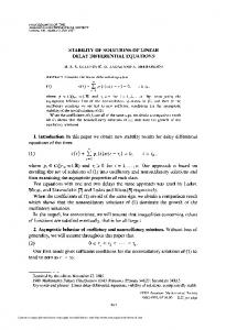
Table II shows the values, for k = −1, 0, 1, for Qk , ˆ k1 and λ ˆ k2 , of Sk . One of Sk , and the eigenvalues, λ the eigenvalues due to the principal branch (k = 0) is closest to the imaginary axis which means that it determines the stability of the system. For the scalar case, (1), it is proved that the root obtained using principal branch always determines the stability of the system [11]. Although such a proof is not available in the matrix-vector case, we observe the same behavior in all the examples we have considered. In this case, the value of the real part of the dominant eigenvalue is in the left half plane, and therefore the system is stable. Using the values of Sk from Table II, we obtain the solution, x(t) =  

0.3499 − 4.9801i −0.6253 + 0.1459i 2.4174 + 0.1308i −5.1048 − 4.5592i

· · · + e  0.3055 −1.4150   t 2.1317i −3.3015 +e C0 +  −0.3499 + 4.9801i −0.6253 − 0.1459i  2.4174 − 0.1308i −5.1048 + 4.5592i e

 t

C−1

 t

C1 + · · · (18) The coefficients Ck in (18) are determined from specified preshape functions, e.g., let ½

x1 (t) x2 (t)

¾

½ =

φ1 (t) φ2 (t)

¾

½ =

1 0

|

eS−N (−T )

0

0.2

0.4

0.6

0.8

1

1.2

1.4

1.6

1.8

2

Time, t

Fig. 1. Comparison for example in (17) of results from numerical integration vs. (18) and (21) with one, three, and, seven terms. With more branches the results show better agreement.

and for T = N =1 in our example we obtain, ½ ¾ ½ ¾ 1.3663 + 3.9491i −1.7327 C−1 = , C0 = , −6.5863 ½ 3.2931 + 9.3999i¾ 1.3663 − 3.9491i C1 = 3.2931 − 9.3999i (21) The results are compared to those obtained using numerical integration in Fig. 1, and show good agreement as more branches are used, i.e., as the dimension of matrix, N increases. The key step, which allows the Lambert function approach to be used in (3), is the introduction, in (11) , of the unknown matrix Qk , and the use of (14) to solve for Qk . III. NON-HOMOGENEOUS SYSTEMS A. Scalar Case The non-homogeneous version of the DDE in (1) is

¾ (19)

Thus, for a delay T , we can write the N term approximation [8],   ¯ φ(0)       T ¯   φ(− )   2N   2T ¯ φ(− 2N ) =   ..       .    ¯  φ(−T ) | {z } Φ(T,N )  eS−N 0 ··· T ) S  e −N (− 2N ···  2T )  eS−N (− 2N ···   ..  . ···

0

x(t) ˙ + ax(t) + ad x(t − T ) = bu(t) t > 0 x(t) = φ(t) t ∈ [−T, 0]

(22)

where u(t) is a continuous function representing the external excitation. In [12], the authors present the forced solution to (22) as, Z t x(t) = Ψ(t, ξ)bu(ξ)dξ (23) 0

where the following conditions for Ψ(t, ξ) must be satisfied. a) eS N 0 T

eSN (− 2N ) 2T eSN (− 2N ) .. .

··· {z Ω(T,N )

eSN (−T )

   C−N   C−(N −1)    C−(N −2)   ..   .    CN }

Ck = lim [Ω−1 (T, N ) · Φ(T, N )]k N →∞

            

(20)

∂ Ψ(t, ξ) ∂ξ

= aΨ(t, ξ), t − T ≤ ξ < t

= aΨ(t, ξ) + ad Ψ(t, ξ + T ), ξ < t − T = 1 = 0, ξ > t (24) In [4], it is not indicated how to compute the fundamental function Ψ(t, ξ). Here we present here an approach based upon the Lambert function. First a Ψ(t, ξ) which satisfies the first condition in (24) is b)Ψ(t, t) c)Ψ(t, ξ)

Ψ(t, ξ) = e−a(t−ξ)

(25)

TABLE II I NTERMEDIATE RESULTS FOR COMPUTING THE SOLUTION IN (18) FOR THE EXAMPLE IN (17) " Qk " Sk λki

k = −1 18.8024 + 10.2243i −61.1342 + 23.6812i

6.0782 + 2.2661i 1.0161 + 0.2653i

0.3499 − 4.9801i −1.6253 + 0.1459i 2.4174 + 0.1308i −5.1048 − 4.5592i ( 1.3990 − 5.0935i −4.0558 − 4.4458i

#

"

#

"

k = −1 9.9183 −32.7746 0.3055 2.1317 (

1

aT

)(t−ξ)

,

k = −∞, . . . , ∞ (26)

There are an infinite number of solutions for the infinite branches of the Lambert function. Therefore the complete solution can be written in terms of the summation ∞ X

Ψ(t, ξ) =

0

Ck e

1 T

Wk (−ad T e

aT

)(t−ξ)

(27)

k=−∞

Thus, the fundamental function is a)Ψ(t, ξ) = e−a(t−ξ) , t − T ≤ ξ < t ∞ X 0 aT 1 = Ck e T Wk (−ad T e )(t−ξ) ,

−0.4150 −3.3015

# #

"

18.8024 − 10.2243i −61.1342 − 23.6812i

0.3499 + 4.9801i −1.6253 − 0.1459i 2.4174 − 0.1308i −5.1048 + 4.5592i ( 1.3990 + 5.0935i −4.0558 + 4.4458i

# #

Z

t

σ(t) =

∞ X

η(t) = 0 Z t

Case I 0 ≤ t ≤ T

0

Ck eSk (t−ξ) bu(ξ)dξ

(32)

k=−∞

e−a(t−ξ) bu(ξ)dξ

δ(t) = t−T t

x(t) =

0

e−a(t−ξ) bu(ξ)dξ

(29)

Consequently the Ck can be represented as:

0

0 ¯ k η −1 (T, N ) · (¯ σ − δ)] Ck = lim [¯

(33)

N →∞

Case II t ≥ T

0

t−T

     

e−a(t−ξ) bu(ξ)dξ

Z 0t−T

Consequently, the forced solution is obtained as,

Z

             

where

(28)

x(t) =

       

(31) ξ t

Z

6.0782 − 2.2661i 1.0161 − 0.2653i

computed using the function in (29) and (30):   σ(T )       T   σ(T − )   2N     2T  σ(T −  ) 2N = . ..                 σ(0) 0   C−N  η−N (T ) ··· ηN (T )   0   η−N (T − T ) · · · ηN (T − T )   C −1) 2N 2N    −(N 0  η−N (T − 2T ) · · · ηN (T − 2T )  C 2N 2N   −(N −2)   .. .. ..     . ··· . .   0  η−N (0) ··· ηN (0) C N  δ(T )    T  ) δ(T − 2N   2T δ(T − + 2N )  .  ..     δ(0)

k=−∞

b)Ψ(t, ξ) = 0,

k = −1

"

1.0119 −1.9841

A Ψ(t, ξ) satisfying the second condition in (24) can be obtained using the Lambert function and confirmed by substitution as, Ψ(t, ξ)k = e T Wk (−ad T e

14.2985 6.5735

VIA THE MATRIX LAMBERT FUNCTION

∞ X

Although, due to space limitation, we omit the derivation, using (31)-(33) can be express the forced solution in (29)(30) as a single equation Z t X ∞ 0 x(t) = Ck eSk (t−ξ) bu(ξ)dξ (34)

0

Ck eSk (t−ξ) bu(ξ)dξ

k=−∞ Z t

+

0 k=−∞

e−a(t−ξ) bu(ξ)dξ

t−T

where, Sk =

1 Wk (−ad T eaT ) T

(30)

Hence, the solution becomes Z t X ∞ ∞ X 0 x(t) = C k e Sk t + Ck eSk (t−ξ) bu(ξ)dξ (35) k=−∞

0

Though the calculation is dependent on u(t), the Ck can be

|

{z

free

}

|

0 k=−∞

{z forced

}

1.2

1.2

1

1

Numerical 0.8

numerical

Lambert method (N=7)

Lambert method (N=7)

0.8

0.6

Responses

Responses

0.6 0.4

0.2

0

0.4

0.2

0 −0.2 −0.2

−0.4

−0.4

−0.6

−0.8

0

5

10

−0.6

15

0

5

10

15

20

Time, t

Fig. 2. Total forced response and comparison between the new method and the numerical method. The agreement is excellent. Parameter are a = ad = T = 1 with u(t) defined by (36)

As seen in (35), the total solution of DDEs using the Lambert function has a similiar form to that of ODEs. (Refer to Table I). The coefficients Ck depend on the initial 0 conditions and the preshape function, but the Ck do not. 0 Note that the Ck are determined only by a, b, ad and the delay time T in (22). Example Consider (22), with a = ad = T = 1 and the forcing input u(t)

= cos(t) t > 0 = 0 t ∈ [−T, 0]

(36)

B. Generalization to System of DDEs The non-homogeneous matrix form of the delay differential equation in (3) can be written as ˙ + Ax(t) + Ad x(t − T ) = Bu(t) x(t) ¯ x(t) = φ(t)

t>0 t ∈ [−T, 0]

(37)

where B is an n × r matrix, and u(t) is a r × 1 vector. The particular solution can be derived from (29)-(30) as, Case I 0 ≤ t ≤ T Z

t

e−A(t−ξ) Bu(ξ)dξ

(38)

0

Case II t ≥ T Z

t−T

x(t) = 0

∞ X

0

eSk (t−ξ) Ck Bu(ξ)dξ

k=−∞ Z t

+

e−A(t−ξ) Bu(ξ)dξ

t−T

where, Sk = 0

30

35

40

45

50

1 Wk (−Ad T eAT Q ) − A T

Fig. 3. Total forced response for (42) and a comparison of the new method with numerical integration

case in the previous section, (38)-(39) are combined as Z t X ∞ 0 x(t) = eSk (t−ξ) Ck Bu(ξ)dξ (40) 0 k=−∞

And the total solution is Z ∞ X Sk t x(t) = e Ck + k=−∞

|

{z

forced

The total response is shown in Fig. 2 for the preshape function , φ(t) = 1 and compared to the result obtained by numerical integration.

x(t) =

25

Time, t

(39)

In (39), Ck is a coefficient matrix of dimension n × n and can be calculated in the same way as (31). Like the scalar

}

|

t

∞ X

0 k=−∞

0

eSk (t−ξ) Ck Bu(ξ)dξ (41) {z

}

forced

Example Consider the systems of DDEs with a constant external excitation: ½ ¾ · ¸½ ¾ x˙ 1 (t) 1 −3 x1 (t) = + x˙ 2 · (t) 2 −5 ¸ ½ x2 (t) ¾ ½ ¾ 1.66 −0.697 x1 (t − T ) cos(t) + 0.93 −0.330 x2 (t − T ) 0 (42) Then the solution to (42) with the preshape function in (19) is obtained from (41) and shown in Fig. 3. The differences between our new method with seven terms and the numerical integration are essentially indistinguishable. IV. CONCLUSION In this paper, the Lambert function approach for analysis of linear delay differential equations in [8] is extended to systems of DDEs and to non-homogeneous systems. The solution obtained using the matrix Lambert function is in a form analogous to the state transition matrix in systems of linear ordinary differential equations (see Table I). Free response and forced response for several cases of DDEs are presented in the paper based on this new solution approach and compared with those obtained by numerical integration. To provide a closed form solution to systems of linear DDEs in a form similar to systems of ordinary differential equations is the essential advantage of the presented analytical approach. The solution is in the form of an infinite series of modes which are expressed in terms of the matrix Lambert function. The concept of the state transition matrix in ODEs can be generalized to DDEs using the matrix Lambert function. This suggests that some

analyses used in systems of ODEs, based on the concept of the state transition matrix, can potentially be extended to systems of DDEs. For example, the approach presented based on the matrix Lambert function, may be useful in controller design via eigenvalue assignment for systems of DDEs. Similarly, concepts of observability, controllability, state estimator design and modal decomposition of systems of DDEs may be tractable. The analytical approach using the matrix Lambert function for ’time-varying’ DDEs based on Floquet theory is already being investigated. These, and others, are all potential topics for future research, which can build upon the foundation presented in this paper. R EFERENCES [1] Gorecki H., Fuksa, S., Grabowski, P., and Korytowski, A., Analysis and Synthesis of Time Delay Systems, John Wiley and Sons, PWNPolish Scientific Publishers Warszawa, 1989 [2] R.E. Bellman and K.L. Cooke, Difference-Difference Equations, Academic Press, 1963 [3] Lam, J., ”Model Reduction of Delay Systems Using Pade Approximants,” Int. J. Control, Vol. 57, No. 2, pp. 377-391, 1993 [4] Golub, G. H., and Van Loan, C. F., Matrix Computations, Johns Hopkins Univ. Press, Baltimore, 1989 [5] Falbo, C. E., ”Analytic and Numerical Solutions to the Delay Differential Equations,” Joint Meeting of the Northern and Southern California Sections of the MAA, San Luis Obispo, CA, 1995 [6] Wright, E. M., ”The Non-Linear Difference-Differential Equation,” Q. J. Math., Vol. 17, pp. 245-252, 1946 [7] Wright, E. M, ”The Linear Difference-Differential Equation With Asymptotically Constant Coefficients,” Am. J. Math., Vol. 70, No. 2, pp. 221-238, 1948 [8] Asl, F.M., and Ulsoy, A.G., ”Analysis of a System of Linear Delay Differential Equations,” ASME J. Dynamic Systems, Measurement and Control, Vol. 125, No. 2, pp 215-223, 2003 [9] Corless, R. M, Gonnet, G. H. Gonnet, D.E.G. Hare, and D.J. Jeffrey, ”On Lambert’s W Function”, Technical Report, Dept. of Applied Math., Univ. of Western Ontario, London, Ontario, Canada [10] Lee T. N. and S. Dianat, ”Stability of Time-Delay Systems”, IEEE Trans. Aut. Control, Vol. AC-26, No. 4, pp. 951-953, 1981 [11] H. Shinozaki, Robust Stability Analysis of Linear Time-Delay Systems by Lambert W Function. Master thesis, Dept. Electro. Inform. Sci., Kyoto Institute of Technology, Kyoto, Japan, 2003 [12] Malek-zavarei, M., Jamshidi, M., Time-delay systems, North Holland, New York, 1987