EUSFLAT-LFA 2011
July 2011
Aix-les-Bains, France
Solution of Fuzzy Differential Equations with generalized differentiability using LU-parametric representation Barnabàs BEDE(1) Luciano STEFANINI(2) (1) University of Texas-Pan American, Edinburg, Texas (e-mail:
[email protected]) (2) University of Urbino "Carlo Bo", Urbino, Italy (e-mail:
[email protected]) small, (i) 9f (x0 + h)
Abstract— The paper uses the LU-parametric representation of fuzzy numbers and fuzzy-valued functions, to obtain valid approximations of fuzzy generalized derivative and to solve fuzzy differential equations. The main result is that a fuzzy differential initial-value problem can be translated into a system of in nitely many ordinary differential equations and, by the LU-parametric representation, the in nitely many equations can be approximated ef ciently by a nite set of four ODEs. Some examples are included. Keywords— Parametric Fuzzy Partition, Fuzzy Transform, Smoothing Functions, Fuzzy Numbers
1
H
f (x0 ); f (x0 )
H
h) and
f (x0
f (x0 + h) H f (x0 ) = (2) h f (x0 ) H f (x0 h) 0 = lim = fGH (x0 ); h&0 h lim
h&0
or (ii) 9f (x0 )
H
lim
f (x0 + h); f (x0
f (x0 )
h&0
Introduction
h)
H
f (x0 ) and
f (x0 + h) = (3) ( h) h) H f (x0 ) 0 = fGH (x0 ); ( h) H
f (x0 = lim The present paper aims to combine results of [1] and [2] with h&0 the parametric representation in [6] to obtain a new approxor (iii) 9f (x0 + h) H f (x0 ); f (x0 h) H f (x0 ) and imation results for fuzzy differential equations (FDE) with parametric representation. These results are used for numerif (x0 + h) H f (x0 ) lim = (4) cally solving FDEs under the parametric representation. The h&0 h problem is that a fuzzy initial value problem in general can f (x0 h) H f (x0 ) 0 be translated to a system consisting of in nitely many ODEs. = lim = fGH (x0 ); h&0 ( h) However the systems are uncoupled, we cannot solve in nitely many equations. This is why we have to approximate or (iv) 9f (x0 ) H f (x0 + h); f (x0 ) H f (x0 h) and the solutions of FDEs. Some examples are presented. f (x0 ) H f (x0 + h) = (5) lim We will denote RF the set of fuzzy numbers, i.e. normal, h&0 ( h) fuzzy convex, upper semicontinuous and compactly supported f (x0 ) H f (x0 h) 0 = lim = fGH (x0 ): fuzzy sets de ned over the real line. The standard Hukuhara h&0 h difference (H-difference •H ) is de ned by u •H v = w () u = v + w; while the generalized Hukuhara difference (gHBased on the gH-difference we obtain the following de difference for short) is the fuzzy number w, if it exists, such nition (for interval-valued functions, the same de nition was that suggested in [4] using inner-difference): u •gH v = w ()
or
(i) (ii)
u=v+w . v=u w
(1)
If w = u •gH v exists as a fuzzy number, its level cuts [w ; w+ ] are obtained by w = minfu v ; u+ v + g + + + and w = maxfu v ;u v g for all 2 [0; 1].
2
De nition 2: Let x0 2]a; b[ and h be such that x0 + h 2]a; b[, then the gH-derivative of a function f :]a; b[! RF at x0 is de ned as 1 0 fgH (x0 ) = lim [f (x0 + h) •gH f (x0 )]: h!0 h
0 If fgH (x0 ) 2 RF satisfying (6) exists, we say that f is generalized Hukuhara differentiable (gH-differentiable for short) at x0 . De ne
Fuzzy differentiability
The following fuzzy differentiability concepts used are of generalized type. The rst concept was presented in [1] for the fuzzy case and the second in [5].
h f (x0 )
De nition 1: ([1]) Let f :]a; b[! RF and x0 2]a; b[: We say that f is strongly generalized Hukuhara differentiable at x0 (GH-differentiable for short) if there exists an element 0 fGH (x0 ) 2 RF ; such that, for all h > 0 suf ciently © 2011. The authors - Published by Atlantis Press
(6)
=
1 [f (x0 + h) •gH f (x0 )]. h
According to the de nition of gH-difference (1), we have two possibilities: (i) 785
h
h f (x0 )
+ f (x0 ) = f (x0 + h)
(7)
(ii)
f (x0 + h)
h
h f (x0 )
= f (x0 ).
(8)
If the limit in (6) exists, we say that f is (i)-gHdifferentiable at x0 (or (ii)-gH-differentiable at x0 ) if (i) is true (or (ii) is true, respectively) for small positive and negative values of h. If only the left-limit (i.e., for h ! 0 , h < 0) in (6) exists, we say that f is (i)-leftgH-differentiable (or (ii)-left-gH-differentiable, respectively) at x0 if equality (7) is valid (or (8) is valid, respectively) for small negative values of h; analogously, we de ne (i)-right-gH-differentiability and (ii)-right-gH(i) lef t - right -gH derivatives are differentiability. The (ii) de ned accordingly.
provided that the 0 two functions (fgH (x)) = minf(f )0 (x); (f + )0 (x)g and 0 (fgH (x))+ = maxf(f )0 (x); (f + )0 (x) de ne (w.r.t. ) a fuzzy number; here, (f )0 ; (f + )0 denote the derivatives w.r.t. x, for given 2 [0; 1]. As f (x) and f + (x) de ne the -cuts of the fuzzy number f (x) for each x, clearly they are monotonic and almost everywhere differentiable w.r.t. and satisfy the conditions of Lemma 1. Assume, for simplicity of presentation, that each function ! f (x) and ! f + (x) is differentiable w.r.t. .
Notation: We will use the following notations: f (x) = @ + @ @ + 0 @ f (x), f (x) = @ f (x), (f ) (x) = @x f (x), @ + 0 (f ) (x) = @x f (x), and, for short, given a fuzzy valThe Lower-Upper (LU) representation of a fuzzy number is ued function f (x), we will denote by f (x) the pairs of a result based on the well known Negoita-Ralescu represenfunctions ( f (x); f + (x)) 2[0;1] ; we will assume that tation theorem, stating essentially that the membership form the following equalities hold for the mixed derivatives: and the -cut form of a fuzzy number u are equivalent and in particular, the -cuts [u] = [u ; u+ ] uniquely represent @ @ ( f )0 (x) = f (x) (9) u, provided that the two functions ! u and ! u+ , @x @ w.r.t. , are left continuous for all 2]0; 1], right continu@ @ = f (x) = (f )0 (x) ous for = 0, monotonic (u increasing, u+ decreasing) and @ @x + u1 u1 (for = 1). @ @ + On the other hand, it is well known that monotonic func( f + )0 (x) = f (x) (10) @x @ tions have at most a countable number of points of discontinuity and a countable number of points where the derivative @ + @ f (x) = (f + )0 (x) . = does not exist. @ @x Denote the corresponding points by the increasing sequence ( j )j2J with 0 < j 1 and J = ; (empty set) or J = f1; 2:::; pg ( nite set) or J = N (set of natural numbers). Then the two functions u ; u+ are differentiable internally The following theorem can be proved. to each of the subintervals ] j 1 ; j [ i.e., they are formed by a family of differentiable monotonic "pieces" (their restrictions Theorem 1: Let f :]a; b[! RF be de ned in terms of its cuts [f (x)] = [f (x); f + (x)] satisfying conditions (9)to each subinterval are monotonic and differentiable). (10). Then For simplicity, in this presentation we will assume that J = 1. f is (i)-gH-differentiable at x if and only if: ; (empty set); otherwise, we can repeat the following results on each of the subintervals. 8 < (f1 )0 (x) (f1+ )0 (x) So, u is assumed to be a fuzzy number with -cuts [u] = for all 2 [0; 1]; ; (11) ( f )0 (x) 0 !u , ! u+ monotonic and differen[u ; u+ ] and : + 0 ( f ) (x) 0 tiable w.r.t. . For 2 [0; 1], let u and u+ denote the rst derivatives 2. f is (ii)-gH-differentiable at x if and only if: of u and u+ w.r.t. (for = 0 they are right derivatives, for 8 = 1 they are left derivatives). < (f1 )0 (x) (f1+ )0 (x) The following lemma is immediate. for all 2 [0; 1]; . (12) ( f )0 (x) 0 : Lemma 1: The two differentiable functions u ; u+ de ne a ( f + )0 (x) 0 fuzzy number if and only if for all 2 [0; 1] we have: 8 8 u+ u+ < u < u De nition 3: A switching point x0 2]a; b[ is such that gHu 0 u 0 . OR : : differentiability changes from type (i) to type (ii) of from u+ 0 u+ 0 type (ii) to type (i). A switching interval ]x0 ; x1 [ is such that x0 < x1 and f is gH-differentiable on its left and on The lemma above is useful to characterize the gHit right but not for all x 2]x0 ; x1 [. differentiability of a fuzzy-valued function f :]a; b[! RF de+ ned in terms of its -cuts [f (x)] = [f (x); f (x)]. Based on the results established in [5], when both f (x) Clearly, by the use of Theorem 2 below, it is easy to nd and f + (x) are differentiable w.r.t. x for all 's, then the - switching points or the starting point of switching intervals. cuts of the gH-derivative of f are Theorem 2: Let f :]a; b[! RF be de ned in terms of its 0 fgH (x) = [minf(f )0 (x); (f + )0 (x)g; cuts [f (x)] = [f (x); f + (x)] satisfying conditions (9)maxf(f )0 (x); (f + )0 (x)g] (10); let f be gH-differentiable; let x0 2]a; b[ be given
3
LU-parametric representation
786
and let > 0 suf ciently small such that x0 2]a; b[ and x0 + 2]a; b[. 1) if conditions (11) hold for x0 < x < x0 and not for x = x0 then x0 is a switching point or the left point of a switching interval. 2) if conditions (12) hold for x0 < x < x0 and not for x = x0 then x0 is a switching point or the left point of a switching interval. 3) if conditions (11) hold for x0 < x < x0 + and not for x = x0 then x0 is a switching point or the right point of a switching interval. 4) if conditions (12) hold for x0 < x < x0 + and not for x = x0 then x0 is a switching point or the right point of a switching interval.
4
3
2
1
0
0
0.1
0.2
0.3
0.4
0.5
0.6
0.7
0.8
0.9
1
0
0.1
0.2
0.3
0.4
0.5
0.6
0.7
0.8
0.9
1
1.5
1
0.5
0
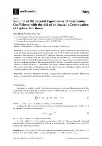
0 Figure 1. f (x) (top) and fgH (x) (bottom) for function in example 1.
In the light of using the results above in the setting of Example 1: Consider the fuzzy valued function f : [0; 1] ! fuzzy differential equations, the LU-parametric representation RF de ned by of fuzzy numbers proposed in [6], is shown to have a great application potential. We will recall here its basic elements. 2 First, we choose a family of "standardized" differentiable f (x) = xe x + 2 (e x + x xe x ) 2 2 and increasing shape functions p : [0; 1] ! [0; 1], depending 2 f + (x) = e x + x + (1 )(ex x + e x ) on two parameters 0 ; 1 0 such that 1. p(0) = 0, p(1) = 1, 0 2. p (0) = 0 , p0 (1) = 1 and We have the following derivatives w.r.t. x of f (x) and 3. p(t) is increasing on [0; 1] if and only if 0 ; 1 0. f + (x) As an example of valid shape functions we can consider rational splines (f )0 (x) = (1 x)e x + t2 + 0 t(1 t) 2 : p(t; 0 ; 1 ) = + 2 (1 2xe x e x + xe x ) 1 + ( 0 + 1 2)t(1 t) + 0 x2 + (f ) (x) = 1 2xe Then, the parametric shape functions above are adopted to 2 2 +(1 )(ex 1 2xe x ) represent the functions u(:) and u+ (:) as "piecewise" differentiable, on a decomposition of the interval [0; 1] into N subintervals 0 = 0 < 1 < ::: < i 1 < i < ::: < N = 1: and the following derivatives w.r.t. At the extremal points of each subinterval Ii = [ i 1 ; i ], the values and the rst derivatives (slopes) of the two functions 2 are given f (x) = 2 (e x + x xe x ) f + (x)
2 (ex
=
x+e
x2
).
u(
i
= u1;i ,
i
1)
= d0;i ,
u0(
i)
= d1;i ,
u0(
( f )0 (x)
=
( f + )0 (x)
=
2 (1 2 (ex
2xe 1
x2
e 2xe
x x2
+ xe ).
x
)
= u0;i , u+ ( i
i)
u( It follows that
1)
1)
= u+ 0;i ,
+ u+ ( i ) = u1;i + u0+ ( i 1 ) = d0;i + u0+ ( i ) = d1;i
,
(13) (14)
and by the transformation t = i ii 11 ; 2 Ii ; each subinterval Ii is mapped into [0; 1] to determine each piece independently. Globally continuous or more regular C (1) fuzzy numbers can be obtained directly from the values of the parameters. Let pi (t) denote the model functions on Ii ; we obtain, for + + example, pi (t) = p(t; 0;i ; 1;i ), p+ i (t) = p(t; 0;i ; 1;i ) i i 1 with j;i = u i ui 1 dj;i and + d+ for j = j;i = u+ u+ j;i
At the point x = 0, f is (ii)-right-gH-differentiable and it is (ii)-gH-differentiable on the interval ]0; x1 [ where x1 = 0:6103336260 is such that (f1 )0 (x1 ) = (f0+ )0 (x1 ); on the interval [x1 ; x2 ], where x2 = 0:7105062170 is such that 1;i 0;i 1;i 0;i (f1+ )0 (x2 ) = (f0 )0 (x2 ), the function is not gH0; 1 so that, for 2 [ i 1 ; i ] and i = 1; 2:; ; ; N : differentiable; f returns to be (i)-gH-differentiable on the interval ]x2 ; 1[; nally, at x = 1 f is (i)-leftu = u0;i + (u1;i u0;i )pi t ; 0;i ; 1;i gH-differentiable. The interval [x1 ; x2 ] is a switching + + + + u+ = u+ u+ 0 0;i + (u1;i 0;i )pi t ; 0;i ; 1;i : interval. Figure 1 shows f and fgH . 787
(15) (16)
A fuzzy number with differentiable lower and upper functions continuous, the differential equation (22) is equivalent to the is obtained by taking the values and the slopes in appropriate following integral equation + + way, i.e. u1;i = u0;i+1 =: ui , u+ 1;i = u0;i+1 =: ui and, for Zt + + the slopes, d1;i = d0;i+1 =: ui , d1;i = d0;i+1 =: u+ i . This f (s; x(s))ds: (23) x(t) • x = gH 0 requires 4(N + 1) parameters, being N 1, t0
+ u = ( i ; u i ; ui ; u + i ; ui )i=0;1;:::;N with
u0
u1
ui
0; u+ i
:::
u+ N
uN
u+ N
1
:::
(17) u+ 0
(18)
If we write (23) in terms of level cuts, we obtain
and the branches are computed according to (15)-(16). The gH-difference w = u •gH v has the following LUparametric form: u •gH v = ( i ; wi ; wi = minfui 0
wi =
wi+ = maxfui 0
4
wi+ =
wi ; wi+ ; vi ; u+ i ui u+ i vi ; u+ i ui u+ i
wi+ )i=0;1;:::;N vi+ g;
vi vi+
x (t) = (x0 ) + x+ (t) = (x0 )+ +
case (ii):
x (t) = (x0 ) + x+ (t) = (x0 )+ +
where
with
if wi = ui if wi = u+ i
vi+ g
vi vi+
case (i):
(19)
0, i = 0; 1; :::; N
if wi+ = ui if wi+ = u+ i
(t; x ; x+ )
=
Rt
+ +
(t; x ; x+ ) (t; x ; x+ ) (t; x ; x+ ) (t; x ; x+ )
f (s; x ; x+ )ds
and
t0 +
(t; x ; x+ ) =
Rt
f + (s; x ; x+ )ds. In both cases, the two
t0
vi vi+
integral equations above are independent for different values of 2 [0; 1], and are equivalent to the ordinary differential equations
vi : vi+
(i):
FDEs with LU-parametric approximation
(ii):
(x )0 = f (t; x ; x+ ); x (t0 ) = (x0 ) (x+ )0 = f + (t; x ; x+ ), x+ (t0 ) = (x0 )+ (x )0 = f + (t; x ; x+ ), x (t0 ) = (x0 ) . (x+ )0 = f (t; x ; x+ ), x+ (t0 ) = (x0 )+ :
Fuzzy differential equations can be considered now with different concepts of differentiability. Using the H-derivative, we As a nal step, we represent all the fuzzy quantities by the can consider the classical Hukuhara differential equation LU-fuzzy parametrization, with the meaning of the symbols as in (17); for each = i and i = 0; 1; :::; N we obtain the x0H = f (t; x); x(t0 ) = x0 ; (20) differential equations with the GH derivative we can consider the problem x0GH = f (t; x); x(t0 ) = x0 ;
(i): (21)
( xi )0 = fi (t; xi ; x+ xi (t0 ) = ( x0 )i i ); + + + + 0 ( x+ ) = f (t; x ; x ), x i i i i i (t0 ) = ( x0 )i
with the gH-derivative we have the equation x0gH = f (t; x); x(t0 ) = x0 :
(xi )0 = fi (t; xi ; x+ i ), xi (t0 ) = (x0 )i + + + + 0 (x+ ) = f (t; u ; u i i i i ), xi (t0 ) = (x0 )i
(22)
(ii):
(xi )0 = fi+ (t; xi ; ux+ i ); xi (t0 ) = (x0 )i + + 0 (x+ ) = f (t; u ; u x+ i i i i ), i (t0 ) = (x0 )i
Everywhere f :]a; b[ RF ! RF is a given function de ned ( xi )0 = fi+ (t; xi ; x+ i ), xi (t0 ) = ( x0 )i in terms + 0 + + + ( x ) = f (t; x ; x i i i i ), xi (t0 ) = ( x0 )i : of level cuts [f (t; x)] = [f (t; x ; x+ ); f + (t; x ; x+ )], [x(t)] = [x (t); x+ (t)]. They are N + 1 independent (systems) of ordinary differential equations (four equations) with given initial conditions; Assumption A: We x a decomposition 0 = 0 < 1 < they can be solved by any of the existing ef cient methods for ::: < i 1 < i < ::: < N = 1 into N subinter- ODE. vals and we obtain an approximation of x(t) and f (t; x) In the following theorem we use the results in [2] to obtain in the form (17); simply, the functions xi (t), x+ i (t) a parametrization of an FDE with GH-derivative. + + + , xi (t), x+ i (t) and fi (t; xi ; xi ), fi (t; xi ; xi ), We denote by D(x; y) the usual Hausdorff distance between + + + fi (t; xi ; xi ), fi (t; xi ; xi ) are computed using (9)- two fuzzy numbers x; y 2 RF . (10) from the level cuts [x(t)] = [x (t); x+ (t)] and For simplicity of notation, the LU-parametric represen[f (t; x)] = [f (t; x ; x+ ); f + (t; x ; x+ )], and for the tations of a fuzzy number x 2 RF and of a function required values of = i , i = 0; :::; N . f (t; x) :]a; b[ RF ! RF as in Assumption A, will be + denoted by xN = ( i ; xi ; xi ; x+ i ; xi ) and fN (t; x) = + + The choice among (20), (21) or (22) of the fuzzy derivative ( i ; f ; f ; f ; f ), respectively; clearly, each of the elei i i i x0 (t) in uences the equation. As we have seen, the deriv- ments f , f , f + and f + can be considered as functions i i i i ative x0 (t) has level cuts [x0 (t)] = [(x )0 (t); (x+ )0 (t)] or of the ve variables t, x , x , x+ and x+ for i = 0; :::; N . i i i i [x0 (t)] = [(x+ )0 (t); (x )0 (t)] when GH or gH differentiability is considered. We analyze the problem (22) at the moment. Theorem 3: Let " > 0 be arbitrary and let x0 2 RF and Following Bede and Gal ([1], Lemma 20), when f (t; x) is f :]a; b[ RF ! RF . Assume that the conditions of 788
Theorem 3.1 in [2] for the solvability of the fuzzy initial The initial condition is x(t0 ) = u where u is a given fuzzy number. value problem We can write the four equations, in terms of gH-derivative, x0 (t) = f (t; x(t)); x(t0 ) = x0 ; (24) as are satis ed. Then there exist LU-parametrizations xN" minf(x (t))0 ; (x+ (t))0 g = (a(t)x(t)) + b (t) 1. and fN" (t; x) with N" subintervals, such that the two somaxf(x (t))0 ; (x+ (t))0 g = (a(t)x(t))+ + b+ (t) lutions of (24) can be approximated with absolute error minf(x (t))0 ; (x+ (t))0 g = (a(t)x(t))+ + b (t) 2. D(x(t); xN" (t)) < " on some interval [t0 ; t0 + k], by maxf(x (t))0 ; (x+ (t))0 g = (a(t)x(t)) + b+ (t) solving the following two sets of ODEs (i = 0; :::; N ): minf(x (t))0 ; (x+ (t))0 g = (a(t)x(t))+ b+ (t) 8 3. 0 + + maxf(x (t))0 ; (x+ (t))0 g = (a(t)x(t)) b (t) > xi = fi (t; xi ; xi ; xi ; xi ) > > 0 > x + + 0 + 0 > = fi (t; xi ; xi ; xi ; xi ) > minf(x (t)) ; (x (t)) g = (a(t)x(t)) + b+ (t) i > < 4. + 0 + + + xi = fi (t; xi ; xi ; xi ; xi ) maxf(x (t))0 ; (x+ (t))0 g = (a(t)x(t))+ + b (t) ; (25) (i) 0 + + + + > > > xi = fi (t; xi +; xi ; xi ;+ xi ) Splitting the four FDE in terms of (i) or (ii) gH> > xi (t0 ) = x0;i ; xi (t0 ) = x0;i > > differentiability, we obtain: : + xi (t0 ) = x0;i ; x+ i (t0 ) = x0;i (x (t))0 = (a(t)x(t)) + b (t) 8 0 1(i) , + + + > xi = fi (t; xi ; xi ; xi ; xi ) (x+ (t))0 = (a(t)x(t))+ + b+ (t) > > 0 > + > xi = fi+ (t; xi ; x+ > i ; xi ; xi ) (x+ (t))0 = (a(t)x(t)) + b (t) > < 1(ii) , + 0 + + xi = fi (t; xi ; xi ; xi ; xi ) (x (t))0 = (a(t)x(t))+ + b+ (t) (ii) . (26) 0 + > x+ = fi (t; xi ; x+ > i i ; xi ; xi ) > > + + > xi (t0 ) = x0;i ; xi (t0 ) = x0;i > (x (t))0 = (a(t)x(t))+ + b (t) > : + , 2(i) xi (t0 ) = x0;i ; x+ (t ) = x 0 i 0;i (x+ (t))0 = (a(t)x(t)) + b+ (t) After the preceding results, the LU parametric representation can be adopted to solve any FDE with fuzzy valued functions having at most a nite number of discontinuities (or points where the derivative w.r.t. does not exist); in fact, it is suf cient that the points b where there is a discontinuity or a non differentiability is included as a point i in the decomposition 0 ::: 1 N of the interval [0; 1] used for the parametric representation. Furthermore, it is possible to intercept the switching points (and the switching intervals) by the following simple rule, based on one of the theorems above. Rule to detect a switching: Consider a time iteration of the FDE solver, i.e. we have evaluated the solution xi (b t b b h); x+ ( t h) at t = t h and we perform the next iteri ation to obtain the solution at t = b t (i.e. with a step size h and assume that the discretization error of the solver is b h) suf ciently small); suppose that xi (b t h) < x+ i (t for all i N ; Solve the systems (25) or (26) starting with i = N and decreasing i from N to 0; b b If, for a given i N , we nd that x+ i (t) < xi (t) then a b b switching point exists between t h and t.
2(ii)
(x+ (t))0 = (a(t)x(t))+ + b (t) , (x (t))0 = (a(t)x(t)) + b+ (t)
3(i)
(x (t))0 = (a(t)x(t))+ + b+ (t) , (x+ (t))0 = (a(t)x(t)) + b (t)
3(ii)
(x+ (t))0 = (a(t)x(t))+ + b+ (t) , (x (t))0 = (a(t)x(t)) + b (t)
4(i)
(x (t))0 = (a(t)x(t)) + b+ (t) , (x+ (t))0 = (a(t)x(t))+ + b (t)
4(ii)
(x+ (t))0 = (a(t)x(t)) + b+ (t) . (x (t))0 = (a(t)x(t))+ + b (t)
Considering that (i)-gH-differentiability requires (x (t))0 (x+ (t))0 8 and (ii)-gH-differentiability requires (x+ (t))0 (x (t))0 8 , we see immediately the following cases, in combination with the necessary validity conditions: (VC): for all t, x1 (t) x+ 1 (t) and, w.r.t. , x (t) is increasing and x+ (t) is decreasing. Observe that equations 1(i) always have an acceptable fuzzy (i)gH-differentiable solution, with increasing support length; equations 1(ii) have an acceptable fuzzy (ii)-gHdifferentiable solution, with decreasing support length, if the 5 Linear fuzzy differential equations validity conditions (VC) are also satis ed; equations Consider the following linear fuzzy differential equations where, for all t 2 [t0 ; T ], a(t) and b(t) are fuzzy num- 2(i) have an acceptable (i)-gH-differentiable solution only if bers having cuts [a(t)] = [a (t); a+ (t)], [b(t)] = (VC) are satis ed and + [b (t); b (t)]: (a(t)x(t))+ + b (t) (a(t)x(t)) + b+ (t); 0 1. x (t) = a(t)x(t) + b(t), equations 2(ii) have an accept2. x0 (t) a(t)x(t) = b(t), able (ii)-gH-differentiable solution only if (VC) are satis ed and 3. x0 (t) a(t)x(t) b(t) = 0, 4. x0 (t)
b(t) = a(t)x(t).
(a(t)x(t)) + b+ (t) 789
(a(t)x(t))+ + b (t);
equations 3(i) cannot have an acceptable fuzzy (i)gH-differentiable solution (unless all is crisp); equations 3(ii) cannot have an acceptable fuzzy (ii)gH-differentiable solution (unless all is crisp); equations 4(i) produce an acceptable (i)-gH-differentiable solution only if (VC) are satis ed and (a(t)x(t)) + b+ (t)
(a(t)x(t))+ + b (t);
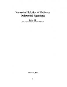
The (ii)-gH-differentiable solution, obtained numerically using the LU-parametric representation with N = 8, is a valid fuzzy number for t 2 [0; t1 ], where t1 0:478; if, at t = t1 , the FDE is switched to (i)-gH-differentiability the solution is continued up to t = 2. The point t1 0:478 is a switching point and the found solution is (ii)-gH-differentiable on [0; t1 ] and (i)-gH-differentiable on [t1 ; 2]. The gH-differentiable solution on the interval [0; 2] is illustrated in Fig. 3. 2
equations 4(ii) produce an acceptable (ii)-gHdifferentiable solution only if (VC) are satis ed and
1.5 1
(a(t)x(t)) + b+ (t)
(a(t)x(t))+ + b (t).
0.5 0
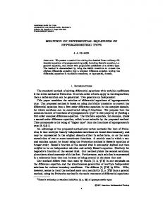
We conclude this section by considering the case of the linear FDE on [a; b] = [0; 2] x0 (t) = (1 t)x(t) + e x(0) = h 0:5; 0:5; 1i
t
-0.5
h0; 0:5; 1i
0
0.2
0.4
0.6
0.8
1
1.2
1.4
1.6
1.8
2
0
0.2
0.4
0.6
0.8
1
1.2
1.4
1.6
1.8
2
2 1
in the case where a(t) = (1 t) is a crisp (non fuzzy) coef cient function and h0; 0:5; 1i is a triangular symmetric fuzzy number with support [0; 1]; we have b (t) = e t 2 and b+ (t) = e t (1 2 ). The initial value (t = 0) is the triangular fuzzy number with support [ 0:5; 1] and core f0:5g. For this equation, the two solutions are obtained by solving two sets of ordinary differential equations, depending on the sign of a(t). The (i)-gH-differentiable solution is obtained by solving the ODEs 8 (1 t)x (t) + e t 2 t 1 > > (x (t))0 = > > (1 t)x+ (t) + e t 2 t > 1 < (1 t)x+ (t) + e t (1 2 ) t 1 (x+ (t))0 = > > (1 t)x (t) + e t (1 2 ) t > 1 > > : x(0) = h 0:5; 0:5; 1i
0 -1 -2
Figure 3. gH-differentiable solution x(t) (top) and its gH-derivative x0gH (t) (bottom).
6
Conclusion
Following the ideas recently developed in [3], we propose here to investigate fuzzy differential equations with gHdifferentiability and we suggest a numerical procedure using the LU-parametric representation.
References and the solution, obtained numerically using the LUparametric representation with N = 8, is the Hukuhara-type [1] B. Bede, S.G. Gal, Generalizations of the differentiabilstandard solution with increasing support (see Fig. 2). ity of fuzzy-number-valued functions with applications to fuzzy differential equations, Fuzzy Sets and Systems, 4 151:581-599, 2005. 2 [2] B. Bede, S.G. Gal, Solution of fuzzy differential equations based on generalized differentiability, Communications in Mathematical Analysis, 9:22-41, 2009.
0 -2 -4
0
0.2
0.4
0.6
0.8
1
1.2
1.4
1.6
1.8
2
4 2
[4] S. Markov, Calculus for interval functions of a real variable, Computing, 22:325-337, 1979.
0 -2 -4
[3] B. Bede, L. Stefanini, Generalized Differentiability of Fuzzy-valued Functions, Submitted for Publication, 1-43, 2011.
0
0.2
0.4
0.6
0.8
1
1.2
1.4
1.6
1.8
2
Figure 2. H-differentiable solution x(t) (top) and its gH-derivative x0H (t) (bottom). The (ii)-gH-differentiable solution is obtained by solving the ODEs 8 (1 t)x+ (t) + e t (1 2 ) t 1 > > > (x (t))0 = > (1 t)x (t) + e t (1 2 ) t > 1 < (1 t)x (t) + e t 2 t 1 . (x+ (t))0 = > + t > (1 t)x (t) + e t > 1 > 2 > : x(0) = h 0:5; 0:5; 1i
[5] L. Stefanini, B. Bede, Generalized Hukuhara differentiability of interval-valued functions and interval differential equations, Nonlinear Analysis, 71:1311-1328, 2009. [6] L. Stefanini, L. Sorini, M.L. Guerra, Parametric representation of fuzzy numbers and application to fuzzy calculus, Fuzzy Sets and Systems, 157:2423-2455, 2006.
790