Hindawi Publishing Corporation International Journal of Aerospace Engineering Volume 2015, Article ID 312430, 6 pages http://dx.doi.org/10.1155/2015/312430
Research Article Solution of Turbine Blade Cascade Flow Using an Improved Panel Method Zong-qi Lei and Guo-zhu Liang Department of Aerospace Propulsion, Beijing University of Aeronautics and Astronautics, Beijing 100191, China Correspondence should be addressed to Zong-qi Lei;
[email protected] Received 27 September 2015; Revised 19 November 2015; Accepted 22 November 2015 Academic Editor: Linda L. Vahala Copyright © 2015 Z.-q. Lei and G.-z. Liang. This is an open access article distributed under the Creative Commons Attribution License, which permits unrestricted use, distribution, and reproduction in any medium, provided the original work is properly cited. An improved panel method has been developed to calculate compressible inviscid flow through a turbine blade row. The method is a combination of the panel method for infinite cascade, a deviation angle model, and a compressibility correction. The resulting solution provides a fast flexible mesh-free calculation for cascade flow. A VKI turbine blade cascade is used to evaluate the method, and the comparison with experiment data is presented.
1. Introduction The design of modern aeroengine gas turbine adopts various numerical methods to increase design efficiency. At the preliminary design stage, the major work for numerical method is repetitive calculations of flow fields over a wide range of blade geometries. This task has been dominated by field methods such as finite differential methods and finite element methods with the advent of computers. However, the use of these field methods requires an experienced user to generate a body-fitted mesh, which is labor intensive. On the other hand, panel method only requires boundary meshes that are one dimension lower than the flow field, reducing the work and difficulty for mesh generation enormously. This method is based on boundary integral equation: it formulated the flow about arbitrary configurations as integration of analytic solutions of singularity distribution over boundary surface [1]. It was initially developed for incompressible potential flow [2]. Soon, the implement of linearised potential equation endowed the method with the capability of solving subsonic and supersonic external flow [3]. Various panel methods were developed using different kind of singularities and higher order panel elements since then eventually evolved into series of computer codes commonly in industrial use [4–7]. The main drawback of the panel method is the limitation of its application to linear potential flow. To be specific, the flow should either be incompressible or possess a sole free
stream as linearization reference. But modern aeroengine gas turbines generally work at high subsonic/transonic condition and adopt blades with large deflection, implying that (1) the incompressible assumption is not applicable and (2) the free streams upstream and downstream of the blades are quite different. There are two schemes to overcome this restriction: the field panel method that uses a field mesh to account for nonlinear effects [8] or the correction correlations that transform the incompressible solution to compressible solution. Since the aim of this paper is to develop a mesh-free method, the correction correlations are chosen as the scheme to be used. There are several forms of corrections based on free stream Mach number [2]. Their combination with the panel method is straightforward and reliable [9]. But as mentioned before, the free stream Mach numbers upstream and downstream of aeroengine gas turbine blades are not the same. Lieblein and Stockman developed a correction for this circumstance [10], which is deduced from empirical observation on the compressible flow in a turbine nozzle passage. However, the error of this method is very large at high subsonic Mach number when compared with experiment data. A method to rapidly calculate turbine blade cascade flow is presented in this paper. The flow field is solved with the panel method at first to obtain an incompressible solution. Then, the free stream velocities upstream and downstream are modified with a deviation angle model. The compressible solution is obtained by applying compressibility corrections
2
International Journal of Aerospace Engineering n
y Nodes
Panels t t
Vonset
m+1
Vonset
Vin
m n N−1
𝛼in Vout
2
𝛼out
1 Endpoint Control point
x
Figure 2: Panel representation of blade.
Figure 1: Flow through infinite cascade.
at each cross section with local average Mach number on the cross section as a reference value. Examples are given to demonstrate the capabilities of the method.
2. Modeling Method 2.1. Panel Method. The flow through an infinite cascade is shown in Figure 1. The governing equations and boundary conditions for inviscid incompressible flow through an infinite cascade are as follows: ∇ ⋅ V = 0,
(1)
V ⋅ nblade surface = 0,
(2)
V → Vin
as 𝑥 → −∞.
(3)
The solution is developed using a velocity potential that is the sum of a constant onset velocity potential plus a disturbance induced by the cascade. The quantities of both are unknown: Φ = 𝜙onset + 𝜙dist ,
(4)
V = −∇Φ = Vonset + Vdist ,
(5)
Vonset = constant.
(6)
distributed along the body surfaces and varying the strength of the source and vortex singularities so that the problem’s boundary conditions are satisfied. In this paper, the surface of the body is represented by inscribing a polygon as shown in Figure 2. Flat panel elements with constant source and vortex singularity strengths are used for simplicity. The source strength varies for each element, while the vortex strength is identical over the whole blade surface. A control point is selected on each element centroid where the normal velocity boundary condition is to be applied. There will be 𝑁 element endpoints and 𝑁 − 1 control points. All the endpoints are arranged clockwise. The trailing edge is left open to avoid a velocity peak in the inviscid calculation. The variables n and t are the unit normal and tangent vectors of the local panel elements, respectively. The velocity in the flow field could be expressed in complex form as follows:
∇ ⋅ Vdist = ∇ 𝜙dist = 0.
(7)
The flow field is determined by solving (1) subject to boundary conditions (2) and (3). Laplace’s equation governs the disturbance potential (7). Since it is a linear equation, simpler solutions of Laplace’s equation may be added together to develop solutions with higher complexity. A general solution to flow over a body or cascade of bodies may be developed by using basic incompressible potential flow solutions for source and vortex flows
𝑁
𝑁
𝑗=1
𝑗=1
V = 𝑉𝑥 − i𝑉𝑦 = ∑ 𝜎𝑗 A𝑗 + 𝛾 ∑ B𝑗 + Vonset ,
(8)
where 𝜎𝑗 is the source strength on the 𝑗th panel element and 𝛾 is the vortex strength over blade surface. A𝑗 and B𝑗 are complex influence factors of the source and vortex at the 𝑗th panel element. According to Hess and Smith [11], their expressions are
The onset velocity is constant, so (1), (5), and (6) yield 2
N
A𝑗 = −
sinh [(𝜋/pitch) [𝑧𝑗+1 − 𝜁]] 𝑒−i𝛽 ), ln ( 2𝜋 sinh [(𝜋/pitch) [𝑧𝑗 − 𝜁]]
(9)
B𝑗 = iA𝑗 , where 𝑧𝑗 , 𝑧𝑗+1 are the endpoints of the 𝑗th element, 𝛽 is the argument of 𝑑𝑧 = 𝑧𝑗+1 − 𝑧𝑗 , 𝜁 is the evaluated point, and pitch stands for the value of pitch. Applying (2) at those control points would yield V𝑖 ⋅ n𝑖 = 0 𝑖 = 1, . . . , 𝑁.
(10)
International Journal of Aerospace Engineering
3
Another boundary condition is the upstream boundary condition (3). For a nominalized velocity field, the inlet velocity could be expressed as follows: Vin = cos 𝛼in − i sin 𝛼in .
P
P
(11)
If the circulation over the blade is Γ (the sum of the vortex strength over the blade), its equation is
Min
𝛼ref
S
𝛼in
Mref
𝑁
Γ = 𝛾 ∑ 𝑙𝑗 ,
S
𝑗=1
(12)
Γ Vin = 𝑉𝑥in − i𝑉𝑦in = 𝑉𝑥onset − i (𝑉𝑦onset + ), 2pitch
𝛼out
where 𝑙𝑗 is the length of the 𝑗th panel element. So the upstream boundary condition could be expressed as 𝑉𝑥in = cos 𝛼in 𝑉𝑦in = 𝑉𝑦onset +
Figure 3: Cross section for compressibility correction.
𝛾 ∑𝑁 𝑗=1 𝑙𝑗 2pitch
(13) .
For airfoil inviscid calculations, a Kutta condition must be applied at the trailing edge: (V1 ⋅ t1 ) + (V𝑁 ⋅ t𝑁) = 0.
(14)
Equations (10), (13), and (14) compose a linear equation group that would yield the values of the singularity strength and Vonset , from which the velocity at any position can be obtained by (8). 2.2. Compressibility Correction. Lieblein’s correction for internal flow is based on the flow status of each cross section: 𝑉𝑐 = 𝑉𝑖 (
𝜌𝑖 ) 𝜌𝑐
𝑉𝑖 /𝑉𝑖
.
(15)
Lieblein’s formula was derived from empirical observation over a turbine nozzle [10]. As shown later in the paper, this does not match with experimental data well. However, this formula indicates the importance of considering the status of local flow paths in the compressibility correction correlations. Thus, a new compressibility correction is developed in this paper: a reference Mach number at the evaluated cross section is calculated first and then is used to transform the local incompressible solution into a compressible solution using the formula for small disturbance flow, such as Karman-Tsien formula: 𝐶𝑝 =
Mout
𝐶𝑝0 2 + (𝑀2 / (1 + √1 − 𝑀2 )) (𝐶𝑝 /2) √1 − 𝑀∞ 0 ∞ ∞
. (16)
Assume there is a virtual flow path where the blade thickness is neglected, and the mass flow rate and average flow angle are equal to those of real blades, as shown in Figure 3 with dash-dotted line. 𝑆𝑃 is the cross section in the flow path where the compressibility correction to be applied, 𝑆 𝑃 , is the cross
section of that virtual flow path at the same axial location. 𝛼ref and 𝑀ref are the average flow angle and the average Mach numbers at 𝑆 𝑃 . According to mass conservation, there is 2 1 + ((𝑘 − 1) /2) 𝑀out ( ) 2 1 + ((𝑘 − 1) /2) 𝑀ref
1/(𝑘−1)
𝑀ref cos 𝛼out = . 𝑀out cos 𝛼ref
(17)
When 𝑀ref is calculated using (17), (16) may be used to transform incompressible solutions into compressible solutions. 2.3. Deviation Angle Model. Equation (17) indicates that the exit flow angle 𝛼out must be obtained in advance to calculate 𝑀ref . However, in practice, the downstream boundary condition is usually back pressure 𝑝out or exit Mach number 𝑀out rather than 𝛼out . The panel method mentioned above is only able to provide the incompressible exit flow angle, the value of which is obviously different from compressible flow. Under this circumstance, a deviation angle model based on momentum balance is introduced to calculate 𝛼out . Consider the pressure distribution on the suction and pressure surface of a turbine blade row flow path shown in Figure 4. The circumferential momentum equation of control volume 𝐴𝐵𝐶𝐷𝐸 is 𝐷
𝐸
𝐶
𝐷
Δ𝐹𝑐 = ∫ 𝑝 𝑑𝑦 − ∫ 𝑝 𝑑𝑦 = Δ (𝑚𝑉)𝑐
(18)
= 𝑚̇ (Vout sin 𝛽out − V𝑜 sin 𝛽op ) . Assume that Δ𝐹𝑦 ≡ 0; thus, there is Vout sin 𝛽out = V𝑜 sin 𝛽𝑜 .
(19)
From the continuity equation, pitch 𝜌out Vout cos 𝛽out = Vop 𝜌op OP, where OP is the opening width, the length of 𝐶𝐷.
(20)
4
International Journal of Aerospace Engineering Table 1: Blade parameters. Parameter Pitch/chord Install angle 𝛽𝑠 Inlet flow angle 𝛼in
D
C 𝛼op
𝛽s
B
Vop p
Ch ord
𝛼in
𝛼out
E Suction surface
Value 0.71 33∘ 30∘
Vout A
pD
pC = pE
Pitch Pressure surface x
Figure 4: Control volume.
The expansion from 𝐶𝐷 to 𝐴𝐵 is assumed to be isentropic. According to the compressible version of Bernoulli’s equation, (
Vop Vout
2
) =
𝑝op (𝑘−1)/𝑘 2 (1 − ( ) ) + 1. 𝑝𝑒 (𝑘 − 1) 𝑀𝑒2
(21)
Reorganizing (19), (20), and (21) yields 2
((
sin 𝛼out 𝑘−1 2 ) − 1) 𝑀𝑒 sin 𝛼op 2
sin 𝛼op pitch 𝑘−1 =1−( ) . tan 𝛼out OP
(22)
Since 𝛼op and pitch/OP can be obtained from the blade geometry, (22) can be solved numerically to provide 𝛼out .
3. Comparison of Results VKI LS 59 turbine cascade data [12] is used to evaluate the modeling method for that its geometry and working condition are similar to those of the aeroengine turbine blades. Lieblein’s method is also used for reference. The blade geometry and general parameters are shown in Figure 5 and Table 1. A FORTRAN computer code of the new method was developed for the calculation. The blade was approximated with 50 elements and the solution required less than 1 second of computer time using a 2.6 GHz Pentium CPU core.
Figure 5: Blade geometry.
3.1. Inlet Mach Number. In Figure 6, the prediction of the inlet Mach number is compared between the new method, Lieblein’s method, and experimental data. As the experiment data shows, the mass flow will not increase with the exit Mach number as the latter approaches unity. The new method shows better consistency with experimental results. 3.2. Exit Flow Angle. The comparison of the exit flow angle is shown in Figure 7. The exit angle of Lieblein’s method does not vary with exit Mach number, since it conserves the mass flow rate of the incompressible solution, which is fixed for a given inlet flow angle, but disagrees with the true value when compressibility effect is strong. In this case, the new method also provides better agreement. 3.3. Surface Mach Number. Figure 8 shows the comparison of the blade surface Mach number distribution. The Mach number given by Lieblein’s method overpredicts the data over the entire blade surface. On the other hand, the new method compares well with the experimental data for the majority of the blade surface.
International Journal of Aerospace Engineering
5
0.35
0.30
Surface Mach number
Inlet Mach number Min
1.0
0.25
0.20
0.15
0.5
0.0
0.3
0.5
0.7 0.9 Exit Mach number Mout
1.1
Present method Lieblein’s method Experiment
0.0
0.2 0.4 0.6 0.8 Axial blade coordinate (x/chord)
1.0
Present method Lieblein’s method Experiment
Figure 6: Inlet Mach number distribution.
Figure 8: Blade surface Mach number distribution.
Conflict of Interests The authors declare that there is no conflict of interests regarding the publication of this paper.
Exit flow angle 𝛼out
70
References 65
60 0.3
0.5 0.7 Exit Mach number Mout
0.9
1.1
Present method Lieblein’s method Experiment
Figure 7: Exit flow angle distribution.
4. Summary The panel method has been adopted to calculate the flow through turbine blades. The inherent computational speed and flexibility of the integral equation solution can make this method useful for design calculations. The method presented combines a panel method, a deviation angle model, and a compressibility correction to yield a compressible solution. Comparison with experiment shows that this method is sufficiently accurate to provide a means of selecting aeroengine turbine blade designs for further analysis.
[1] J. L. Hess, “Panel methods in computational fluid dynamics,” Annual Review of Fluid Mechanics, vol. 22, no. 1, pp. 255–274, 1990. [2] J. L. Hess and A. M. O. Smith, “Calculation of non-lifting potential flow about arbitrary three-dimensional bodies,” E.S. 40622, Douglas Aircraft Division, 1962. [3] F. A. Woodward, “Analysis and design of Wing-Body combinations at subsonic and supersonic speed,” Journal of Aircraft, vol. 5, no. 6, pp. 528–534, 1968. [4] L. Morino, “Oscillatory and unsteady subsonic and supersonic aerodynamics—production version (SOUSSA-P.1,1) vol. 1, theoretical manual,” NASA CR-159130, 1980. [5] R. L. Carmichael and L. L. Erickson, “PAN AIR—a higher order panel method for predicting subsonic or supersonic linear potential flows about arbitrary configurations,” in Proceedings of the 14th Fluid and Plasma Dynamics Conference, AIAA Paper 81-1255, Palo Alto, Calif, USA, 1981. [6] L. Fornasier, “HISS—a higer order subsonic/supersonic singularity method for calculating linearized potential flow,” AIAA Paper 84-1646, 1984. [7] B. Maskew, “Program VSAERO theory document,” NASA CR 4023, 1987. [8] L. Gebhardt, D. Fokin, T. Lutz, and S. Wagner, “An implicitexplicit dirichlet-based field panel method for transonic aircraft design,” in Proceedings of the 20th AIAA Applied Aerodynamics Conference, AIAA 2002-3145, St. Louis, Mo, USA, June 2002. [9] M. Drela, “XFOIL: an analysis and design system for low reynolds number airfoils,” in Low Reynolds Number Aerodynamics, T. J. Mueller, Ed., vol. 54 of Lecture Notes in Engineering, pp. 1–12, Springer, Berlin, Germany, 1989.
6 [10] S. Lieblein and N. O. Stockman, “Compressibility correction for internal flow solutions,” Journal of Aircraft, vol. 9, no. 4, pp. 312– 313, 1972. [11] J. L. Hess and A. M. O. Smith, “Calculation of potential flow about arbitrary bodies,” Progress in Aerospace Sciences, vol. 8, pp. 1–138, 1967. [12] R. Kiock, F. Lehthaus, N. C. Baines, and C. H. Sieverding, “The transonic flow through a plane turbine cascade as measured in four european wind tunnels,” Journal of Engineering for Gas Turbines and Power, vol. 108, no. 2, pp. 277–284, 1986.
International Journal of Aerospace Engineering
International Journal of
Rotating Machinery
Engineering Journal of
Hindawi Publishing Corporation http://www.hindawi.com
Volume 2014
The Scientific World Journal Hindawi Publishing Corporation http://www.hindawi.com
Volume 2014
International Journal of
Distributed Sensor Networks
Journal of
Sensors Hindawi Publishing Corporation http://www.hindawi.com
Volume 2014
Hindawi Publishing Corporation http://www.hindawi.com
Volume 2014
Hindawi Publishing Corporation http://www.hindawi.com
Volume 2014
Journal of
Control Science and Engineering
Advances in
Civil Engineering Hindawi Publishing Corporation http://www.hindawi.com
Hindawi Publishing Corporation http://www.hindawi.com
Volume 2014
Volume 2014
Submit your manuscripts at http://www.hindawi.com Journal of
Journal of
Electrical and Computer Engineering
Robotics Hindawi Publishing Corporation http://www.hindawi.com
Hindawi Publishing Corporation http://www.hindawi.com
Volume 2014
Volume 2014
VLSI Design Advances in OptoElectronics
International Journal of
Navigation and Observation Hindawi Publishing Corporation http://www.hindawi.com
Volume 2014
Hindawi Publishing Corporation http://www.hindawi.com
Hindawi Publishing Corporation http://www.hindawi.com
Chemical Engineering Hindawi Publishing Corporation http://www.hindawi.com
Volume 2014
Volume 2014
Active and Passive Electronic Components
Antennas and Propagation Hindawi Publishing Corporation http://www.hindawi.com
Aerospace Engineering
Hindawi Publishing Corporation http://www.hindawi.com
Volume 2014
Hindawi Publishing Corporation http://www.hindawi.com
Volume 2014
Volume 2014
International Journal of
International Journal of
International Journal of
Modelling & Simulation in Engineering
Volume 2014
Hindawi Publishing Corporation http://www.hindawi.com
Volume 2014
Shock and Vibration Hindawi Publishing Corporation http://www.hindawi.com
Volume 2014
Advances in
Acoustics and Vibration Hindawi Publishing Corporation http://www.hindawi.com
Volume 2014