The gradient problem of C. E. Weil is the following question: Assume n ⥠2 ...... Using that gn(c) is monotone increasing as n â â and it increases infinitely.
Rev. Mat. Iberoamericana 21 (2005), no. 3, 889–910
Solution to the gradient problem of C. E. Weil Zolt´ an Buczolich
Abstract In this paper we give a complete answer to the famous gradient problem of C. E. Weil. On an open set G ⊂ R2 we construct a differentiable function f : G → R for which there exists an open set Ω1 ⊂ R2 such that ∇f (p) ∈ Ω1 for a p ∈ G but ∇f (q) �∈ Ω1 for almost every q ∈ G. This shows that the Denjoy-Clarkson property does not hold in higher dimensions.
1. Introduction The gradient problem of C. E. Weil is the following question: Assume n ≥ 2 and G ⊂ Rn is open, f : G → R is a differentiable function. Then ∇f maps G into Rn . Assume Ω ⊂ Rn is open. Is it true that (∇f )−1 (Ω) = {p ∈ G : ∇f (p) ∈ Ω} is either empty, or of positive n-dimensional Lebesgue measure? When n = 1 then the answer is positive and is the so called DenjoyClarkson property of the derivative functions [8], [7]: If f : (a, b) → R is a differentiable function and (α, β) is an open interval then (f � )−1 (α, β) is either empty, or of positive (one dimensional) Lebesgue measure. In [12] it was shown that the kth Peano derivatives and the approximate derivatives also have the Denjoy-Clarkson property. The gradient problem was one of the well-known and famous unsolved problems in Real Analysis. It was around since the paper [12] appeared in the 1960s. I have learned it in 1987 and have worked on it since then. In 1990 at the Fourteenth Summer Symposium on Real Analysis it was advertised and appeared in print in [13]. 2000 Mathematics Subject Classification: Primary: 26B05. Secondary: 28A75, 37E99. Keywords: Gradient, Denjoy-Clarkson property, Lebesgue measure.
890 Z. Buczolich In this paper we answer this question by giving a two dimensional counterexample. We show that there exists a nonempty open set G ⊂ R2 , a differentiable function f : G → R and an open set Ω1 ⊂ R2 for which there exists a p ∈ G such that ∇f (p) ∈ Ω1 but for almost every (in the sense of two dimensional Lebesgue measure, λ2 ,) q ∈ G the gradient ∇f (q) is not in Ω1 . The result in [2] which was reproved by different methods in [10] shows that in the above example, although λ2 ((∇f )−1 (Ω1 )) = 0, if H1 denotes the one dimensional Hausdorff measure then H1 ((∇f )−1 (Ω1 )) > 0. The results in [10] imply more than this. It turns out that any projection of (∇f )−1 (Ω1 ) onto a line is of positive λ1 measure, (∇f )−1 (Ω1 ) is non-σ-porous and is porous at none of its points. The results in [5] also show that if v is an interior point of def R1 = Ω1 ∩ {∇f (p) : p ∈ G} then H1 ((∇f )−1 (v)) > 0, which implies that (∇f )−1 (Ω1 ) is of non-σ-finite H1 measure. Furthermore, the range R1 satisfies a certain interesting convexity/concavity property. Actually, this convexity/concavity property is behind the construction of the counterexample given in this paper. These results from [5] show that our counterexample function has some strange properties. On the other hand, [3] shows that if ∇f �= (0, 0) on G (this will be true in our counterexample) then the level set structure of f is relatively simple, f −1 ({y}) has components which are homeomorphic to differentiable arcs and there are no bifurcation points on these components. Related to our work on the gradient problem in [6] a pathological C 1 -function, with “too many tangent planes” was constructed. This result pointed in the direction that maybe the counterexample function of this paper exists. In [11] G. Petruska verified that if F : R → R is a differentiable function of one variable and f = F � then f takes each of its values on Af , where Af denotes the approximate continuity points of f . In [4] we showed that if F : Rn → R is differentiable and i ∈ {1, . . . , n} then f = ∂i F takes each of its values on Af . On the other hand, there exists a continuous function F : R2 → R such that f = ∂F/∂x1 exists everywhere and f does not take each of its values on Af . In Theorem 3 of [4] a differentiable function f : R2 → R is constructed such that ∇f does not take each of its values on A∇f . Assume f : Rn → R is a differentiable function. We call a point y ∈ Rn a regular value of ∇f if there is an x ∈ A∇f such that ∇f (x) = y. Denote the set of regular values by REG(∇f ). Our question in [4] about the density of REG(∇f ) in the range of ∇f receives a negative answer by the negative answer to the gradient problem. On the other hand our question about the characterization of REG(∇f ) remains open.
Solution to the gradient problem of C.E. Weil
891
There is a new question related to the gradient problem: Assume that G ⊂ Rn is an open set, f : G → R is a differentiable function and Ω ⊂ Rn is such an open set that (∇f )−1 (Ω) �= ∅. Then what can we say about the Hausdorff-dimension of (∇f )−1 (Ω). The results discussed above imply that (∇f )−1 (Ω) is of Hausdorff dimension at least one, and our counterexample in this paper shows that it is possible that λ2 ((∇f )−1 (Ω)) = 0.
2. Main Result This section is devoted to the proof of our main result, Theorem 1. We put G = (−1, 1)×(−1, 1) and Ω0 = [− 12 , 12 ]×[0, 2], Ω1 = (−0.49, 0.49)× (0, 1.99), and Ω2 = [−0.51, 0.51] × [0, 2.01]. Theorem 1. There exists a differentiable function f : G → R such that ∇f (0, 0) = (0, 1) and ∇f (p) �∈ Ω1 for almost every p ∈ G. The construction of f is quite complicated and is done in Subsection 2.2. Here is an informal plan of what we are doing. We start with a function h−1 (x, y) = y. Then ∇h−1 = (0, 1) everywhere on G. Now our aim is to choose a sequence of functions hn so that def
f (x, y) =
∞ �
hn (x, y)
n=−1
satisfies Theorem 1. Each � function hn+1 can be regarded as a perturbation of the previous partial sum nk=−1 hk . Our aim is to push ∇f (p) outside of Ω1 for almost every p ∈ G. In the construction we will have a nested sequence of open sets Gn such that for almost every p outside of Gn we will have ∇f (p) �∈ Ω1 . We use a “stopping time argument” by not perturbing the function point, p any more, once ∇f (p) �∈ Ω0 . For �∞at almost every� n0 these points n=−1 hn (x, y) = n=−1 hn (x, y) for a suitable n0 . We will show that λ2 (Gn ) → 0. The main difficulty is to show that f is differentiable at those points p ∈ ∩∞ n=0 Gn which are subject to infinitely many perturbations. To handle this difficult case an argument which originates from dynamical systems is used, I learned the heuristic behind this argument when I worked on the proof of [1]. This important argument is discussed first in Subsection 2.1. Reading this subsection one should think that �p is a given point in G and the trajectory xn is the first coordinate of ∇( n−1 k=−1 hk (p)) (apart from some vanishing error term) and yn is the second coordinate (again with some vanishing error term). A sequence {gn } of concave down auxiliary functions is also defined. These functions will determine the way we move in the gradient space and the motivation for the introduction of these functions originates from the convexity/concavity result in [5].
892 Z. Buczolich 2.1. Trajectories in the gradient space, the dynamics behind our construction Set x0 = 0, y0 = 1, a(0, 1) = 0, k0 = 1, A0 = {0}, g0 (x) = 1 − 14 x4 . Suppose n ≥ 0 and the trajectory xk ∈ [−1, 1], for k = 1, . . . , n is given together with another sequence yk ∈ R. This second sequence is computed based on the trajectory {xk }. We also have a set An ={a(n, j) : j = 1, . . . , kn } which gives the indices of the so called active points of the trajectory: xa(n,1) , . . . , xaa(n,kn ) . We assume that a(n, j) < a(n, j +1), j = 1, . . . , kn −1 and a(n,kn ) = n. The point x0 = 0 will always be regarded to be active. Hence a(n, 1) = 0 for all n. We also have a collection of functions gk , k = 1, . . . , n which are concave down and gk (xk ) = yk . We also assume, xj+1 − xj �= 0 for j = 0, . . . , n − 1. Suppose that the next term xn+1 �= xn of the trajectory is given. Denote by τ (x) the tangent of gn at the point (xn , gn (xn )). Set yn+1 = τ (xn+1 ). Since gn is concave we clearly have yn+1 ≥ gn (xn+1 ). See Figure 1. 6
(x2 , y2 ) ... (x1 , y1 ) .
τ (x)
... ................ ... ... ... ... ... ... ... ... ... ... ... ... ... .. .
x1 = xa(1,2)
x2 0 = x0 = xa(1,1)
g1 -
Figure 1: The functions gn .
If the trajectory at step n + 1 is not changing direction, that is, (xn − xn−1 )(xn+1 − xn ) > 0 then xn becomes inactive and this means that it will not belong to An+1 . (At the first step, by definition, we do not change direction.) If the trajectory at step n + 1 is changing direction, that is, (xn − xn−1 )(xn+1 − xn ) < 0 then xn stays active, that is, xn ∈ An+1 , provided it is not decativated by the “passing over” rule given below. The last point of the trajectory xn+1 is always active, so n + 1 = a(n + 1, kn+1 ) ∈ An+1 .
Solution to the gradient problem of C.E. Weil
893
Inactive points cannot become active but some active points might get deactivated when xn is “passing over” them, or over their predecessors. This means that if xa(n,j) ∈ (xn , xn+1 ] for a j ∈ {1, . . . , kn } then all xa(n,j � ) with j ≤ j � ≤ kn , j � �= 1 become inactive and these a(n, j � )’s will not belong to An+1 . If 0 = x0 ∈ (xn , xn+1 ] we say that we are resetting the active trajectory, and An+1 = {0, n + 1} in this case. The elements of An which are not deactivated by the above process will belong to An+1 . The only way xn can survive step n + 1 as an active point is by being a turning point of the trajectory. Hence, all active points are (some earlier) turning points, that is, (xa(n,j) − xa(n,j−1) )(xa(n,j+1) − xa(n,j) ) < 0. Assuming xa(n,2) < xa(n,1) = 0 the “cancellation by passing over” rule implies that we have xa(n,2(j−1)) ≤ xa(n,2j) , xa(n,2j−1) ≥ xa(n,2j+1) and xa(n,2j) ≤ xn ≤ xa(n,2j � −1) for all j, j � for which the arguments of a(n, .) are defined. See Figure 2. In case xa(n,2) > xa(n,1) = 0 we have a mirror image and all inequalities are reversed. xa(n,2) xa(n,4)
xn = xa(n,kn )
xa(n,3)
0 = xa(n,1)
Figure 2: Active points at step n.
If a, b ∈ R we denote the closed interval with endpoints a and b by [a, b] irregardless whether a ≤ b, or b ≤ a, we adopt similar convention for other type of intervals as well. Next we show how gn is defined. We define its derivative gn� on R and assume that it also satisfies the initial condition gn (xn ) = yn . We still assume xa(n,2) < xa(n,1) = 0, the case xa(n,2) > xa(n,1) = 0 is similar, the case xa(n,2) = xa(n,1) = 0 is trivial, we set gn� (x) = −x3 . On [xa(n,1) , +∞) and on (−∞, xa(n,2) ] we put gn� (x) = −(x − xa(n,1) )3 = −x3 . This also defines gn� (xa(n,2) ) = −(xa(n,2) − xa(n,1) )3 . Assume gn� (xa(n,j) ) = −(xa(n,2) −xa(n,1) )3 −(xa(n,3) −xa(n,2) )3 −· · ·−(xa(n,j) −xa(n,j−1) )3 . For a j ∈ {2, . . . , kn − 1} on [xa(n,j+1) , xa(n,j−1) ) we put gn� (x) = gn� (xa(n,j) ) − (x − xa(n,j) )3 . Which implies gn� (xa(n,j+1) ) = −(xa(n,2) − xa(n,1) )3 − (xa(n,3) − xa(n,2) )3 − · · · − (xa(n,j) − xa(n,j−1) )3 − (xa(n,j+1) − xa(n,j) )3 . Finally, on the interval (xa(n,kn −1) , xa(n,kn ) ) put gn� (x) = gn� (xa(n,kn ) ) − (x − xa(n,kn ) )3 . Since gn� (xa(n,kn ) ) = gn� (xa(n,kn −1) ) − (xa(n,kn ) − xa(n,kn −1) )3 the function gn� is continuous at xa(n,kn −1) .
894 Z. Buczolich �
x
We set gn (x) = yn +
gn� (x)dx.
xn
gn�
Observe that is continuous at the points xa(n,j) , j = 1, . . . , kn and is monotone decreasing on the intervals determined by these active points. Hence gn is concave (down) on R. We will only be interested in gn when the trajectory, {xn }, is in [−1, 1] and with this assumption we also have |gn� (x)| ≤ 1 for x ∈ [−1, 1]. Lemma 2. For all x ∈ R and n = 0, 1, . . . we have gn+1 (x) ≥ gn (x). Proof. We separate three cases. Case I: There is no cancellation of active points and at step n + 1 the trajectory is not turning its direction. This implies kn+1 = kn . Case II: There is no cancellation and at step n + 1 the trajectory is changing its direction. Then xn stays active and xn+1 becomes active. Thus kn+1 = kn + 1 > kn . Case III: There is some cancellation of active points. Then kn+1 ≤ kn and kn+1 = kn is possible only when kn+1 = kn = 2 and at step n + 1 we reset the trajectory. During the whole proof we assume xa(n,2) < xa(n,1) = 0, the case xa(n,2) > xa(n,1) = 0 is similar, the case xa(n,2) = xa(n,1) = 0 is trivial. def
Case I: Without limiting generality we can also suppose that u = xa(n,kn −1) = xa(n+1,kn+1 −1) < xn < xn+1 < w = xa(n,kn −2) = xa(n+1,kn+1 −2) ≤ xa(n,1) , see � on (−∞, u] Figure 3. By using the definition of the functions gn and gn+1 � � and on [xn+1 , +∞) we have gn = gn+1 , this might not completely clear on � (xn+1 , w) but on this interval gn� (x) = gn+1 (x) = gn� (u) − (x − u)3 . Thus it is enough to show gn+1 ≥ gn on [u, xn+1 ]. �
-
-
u = xa(n,kn −1) xn = xa(n,kn )
xn+1
w = xa(n,kn −2)
0 = xa(n,1)
Figure 3: Case I. � � On [xn , xn+1 ] we have gn� (x) = gn� (u) − (x − u)3 and gn+1 (x) = gn+1 (xn+1 ) − 3 � 3 3 (x − xn+1 ) = gn (u) − (xn+1 − u) − (x − xn+1 ) . So � (x) − gn� (x) = −(xn+1 − u)3 − (x − xn+1 )3 + (x − u)3 gn+1 = −((xn+1 − x) + (x − u))3 + (xn+1 − x)3 + (x − u)3 < 0,
Solution to the gradient problem of C.E. Weil
therefore, using x < xn+1 we infer
�
x
895
� (gn+1 (t) − gn� (t))dt > 0,
gn+1 (x) − gn+1 (xn+1 ) − (gn (x) − gn (xn+1 )) = xn+1
which based on yn+1 = gn+1 (xn+1 ) ≥ gn (xn+1 ), yields gn+1 (x) ≥ gn (x) for all x ∈ [xn , xn+1 ]. On [u, xn ] we have gn� (x) = gn� (xn ) − (x − xn )3 = gn� (u) − (xn − u)3 − (x − xn )3 and � � � (x) = gn+1 (xn+1 ) − (x − xn+1 )3 = gn+1 (u) − (xn+1 − u)3 − (x − xn+1 )3 gn+1 = gn� (u) − (xn+1 − u)3 − (x − xn+1 )3 .
Now, � (x) − gn� (x) = −(xn+1 − u)3 − (x − xn+1 )3 + (xn − u)3 + (x − xn )3 , gn+1 � (u) − gn� (u) = 0, and gn+1 �� �� gn+1 (x) − gn (x) = −3(x − xn+1 )2 + 3(x − xn )2 < 0. � − gn� ≤ 0 on [u, xn ]. Hence, again Thus gn+1
�
x
gn+1 (x) − gn+1 (xn ) − (gn (x) − gn (xn )) =
� (gn+1 (t) − gn� (t))dt ≥ 0.
xn
Since we have already verified that gn+1 (xn ) ≥ gn (xn ) this implies gn+1 (x) ≥ gn (x) on [u, xn ]. Case II. Now kn+1 > kn . Again, without limiting generality, we assume xn+1 < xn < xa(n,1) = xa(n+1,1) = 0 and setting def
u = xa(n,kn −1) < xn+1
and
def
w = xa(n,kn −2)
we have u < xn+1 < xn < w ≤ xa(n,1) , see Figure 4. Now, by our assumptions xn = xa(n+1,kn ) and xn+1 = xa(n+1,kn +1) . � � u = xa(n,kn −1) xn+1
xn = xa(n,kn )
w = xa(n,kn −2)
Figure 4: Case II.
0 = xa(n,1)
896 Z. Buczolich � On (−∞, u] and on [w, +∞) by our definitions we have gn� = gn+1 . On [xn , w] we have � � (u) − (x − u)3 = gn+1 (x). gn� (x) = gn� (u) − (x − u)3 = gn+1
On [u, xn+1 ] we also have gn� (x) = gn� (xn ) − (x − xn )3 and � � gn+1 (x) = gn+1 (xn ) − (x − xn )3 = gn� (x).
On [xn+1 , xn ], � � (x) = gn+1 (xn+1 ) − (x − xn+1 )3 = gn� (xn ) − (xn+1 − xn )3 − (x − xn+1 )3 , gn+1
and gn� (x) = gn� (xn ) − (x − xn )3 . Hence � (x) − gn� (x) = −(xn+1 − xn )3 − (x − xn+1 )3 + (x − xn )3 gn+1 = ((xn − x) + (x − xn+1 ))3 − (x − xn+1 )3 − (xn − x)3 > 0
and
�
x
gn+1 (x) − gn+1 (xn+1 ) − (gn (x) − gn (xn+1 )) =
� (gn+1 (t) − gn� (t))dt > 0.
xn+1
This, together with yn+1 = gn+1 (xn+1 ) ≥ gn (xn+1 ), implies again that gn+1 (x) ≥ gn (x). Case III. Now kn+1 ≤ kn and there are some deactivated points of the trajectory. First we assume that the trajectory at step n+1 is not changing its direction, this is called Case IIIa. Without limiting generality we can assume xn < xa(n,1) , xn < xn+1 and, due to the cancellation, uj = xa(n,kn −2j) ∈ (xn , xn+1 ] for j = 1, . . . , j0 with some j0 ≥ 1. Set wj = xa(n,kn −2j+1) , j = 1, . . . , j0 . Then wj0 < · · · < w2 < w1 < xn < u1 < · · · < uj0 ≤ xn+1 , see Figure 5. �
-..................................................... -
�
-
� wj0 +1 wj0 w2 w1
xn
u1
Figure 5: Case IIIa.
u2 uj0
xn+1
Solution to the gradient problem of C.E. Weil
897
For t ∈ [xn , xn+1 ] we define some auxiliary functions gn,t . � (x) = gn� (x) for x ≤ w1 or For t ∈ [xn , u1 ) set gn,t (t) = gn (t) and gn,t x ≥ u1 . For x ∈ [t, u1 ) set � � (x) = gn,t (w1 ) − (x − w1 )3 = gn� (w1 ) − (x − w1 )3 = gn� (x). gn,t
See Figure 6. This implies gn,t (x) = gn (x) for all x ≥ t. For x ∈ (w1 , t] set � � � (x) = gn,t (t) − (x − t)3 = gn,t (w1 ) − (t − w1 )3 − (x − t)3 . gn,t
common tangent of gn and gn,t gn,t (x)
.... ... ... ... ... ... ....
w1
gn (x)
... ... .... ... ... ... ... ... ... ... ....
xn
... ... ... ... ... ... ... ... ... ... ... ... ... ..
t
... .... ... ... ... ... ... ... .... ... ... ... ... .. -
u1
Figure 6: The functions gn and gn,t .
Observe that the definition of gn,t is exactly the same what we would have obtained in Case I if we had xn+1 = t and yn+1 = gn (t). So, as in Case I, one could see that gn,t (x) ≥ gn (x) for all x ∈ R. (See Figure 6.) Furthermore, taking t, t� ∈ (xn , u1 ), t < t� and thinking of t as being the next point of the trajectory, xn+1 , and t� as xn+2 , yn+1 = gn (t), yn+2 = gn (t� ) one could see like in Case I that gn,t� (x) ≥ gn,t (x). � � Set Set gn,u−1 (x) = limt→u−1 gn,t (x). Then gn,u − (x) = limt→u− gn,t (x). 1 1 � � n1 = a(n, kn − 2), then u1 = xn1 and next we show that gn,u− (x) = gn1 (x) 1 which shows that after the cancellation at u1 we are “dropping down” to a function which is a vertically shifted copy of gn1 . Indeed, for x �∈ (w1 , u1 ) � � � we have gn,u − (x) = gn (x) = gn1 (x). For x ∈ (w1 , u1 ) we have 1
� � 3 � 3 gn,u − (x) = gn (u1 ) − (x − u1 ) = gn (u1 ) − (x − u1 ) . 1 1
It is also clear that gn,u−1 (x) ≥ gn (x). Again we want to reduce our argument to Case I. Here is the idea of what we are planning to do: Due to cancellation we can forget the trajectory xn for n > n1 and when studying gn,t for t ∈ [u1 , u2 ) we can use the argument from Case I with yn1 = gn,u−1 (xn1 ), xn1 +1 = t and yn1 +1 = gn,u−1 (t).
898 Z. Buczolich Furthermore, like in the earlier case, we can also obtain the monotonicity property for all t, t� ∈ [u1 , u2 ), t < t� and x ∈ R.
gn,t� (x) ≥ gn,t (x)
(2.1)
So assume t ∈ [u1 , u2 ) and set gn,t (t) = gn,u−1 (t) = gn (t). For x ≥ t, or for x ≤ w2 set � � � � (x) = gn,u gn,t − (x) = gn (x) = gn (x). 1 1
This again implies gn,t (x) = gn (x) for x ≥ t. For w2 < x < t set � � (x) = gn,t (t) − (x − t)3 = gn� 1 (t) − (x − t)3 . gn,t
Now, as earlier, by using an argument similar to Case I (now applied for gn1 (t)) one could see that gn,t (x) − gn,t (t) − (gn1 (x) − gn1 (t)) ≥ 0 for w2 < x < t and hence gn,t (x) ≥ gn,u−1 (x) for all x ∈ R. The monotonicity property (2.1) can be established as well. Then one can define gn,u−2 (x) and continue the argument on [u2 , u3 ). By induction we can prove (2.1) for all intervals [ul−1 , ul ) for l = 2, . . . , j0 and setting nl = a(n, kn − 2l) we have gn,u− (x) = gn� l (x) on R. l Hence we can define gn,u−j (x) and 0
� gn,u − j
0
(x) =
gn� (uj0 )
− (x − uj0 )3 = gn� j0 (uj0 ) − (x − uj0 )3
� � � on (wj0 , uj0 ) while gn,u − (x) = gnj (x) = gn (x) for x �∈ (wj0 , uj0 ). 0 j0
Set wj0 +1 = xa(n,kn −2j0 −1) if kn − 2j0 − 1 ≥ 1. If kn − 2j0 − 1 < 1 then xa(n,1) = x0 = 0 ∈ (xn , xn+1 ] and at step n + 1 we reset the trajectory. In this case uj0 = 0 and we put wj0 +1 = 0. We also � � 3 have gn,u − (x) = g0 (x) = −x and gn,u− (0) = gn,uj (uj0 ) = gn (0). 0 j j0
0
Now we return to the proof of this lemma and no longer assume uj0 = 0. � For t ∈ [uj0 , xn+1 ] we define gn,t (t) = gn (t) and gn,t (x) = gn� j0 (x) = gn� (x) � � when x �∈ (wj0 +1 , t). When x ∈ (wj0 +1 , t) set gn,t (x) = gn,t (t) − (x − t)3 . The monotonicity property (2.1) can be established as before. Hence gn,xn+1 (x) ≥ gn,t (x) ≥ gn,u−j (x) ≥ · · · ≥ gn (x) for all x ∈ R. 0
� � Now, gn+1 (xn+1 ) > gn (xn+1 ) = gn,xn+1 (xn+1 ) and gn+1 = gn,x implies n+1 gn+1 ≥ gn . In the proof of Lemma 4 we need the following estimate for the case when uj0 = 0, that is, when we reset the trajectory: � x x4 (2.2) gn+1 (x) ≥ gn,u−j (x) = gn,u−j (0) + −t3 dt = gn (0) − 0 0 4 0 (we remark that this inequality holds in Case IIIb as well, provided that uj0 = 0).
Solution to the gradient problem of C.E. Weil
899
Case IIIb. Now we assume that at step n + 1 the trajectory is changing direction. The other cases being similar we assume xn < xa(n,1) , xn < xn+1 , xn < xn−1 . Set u1 = xa(n,kn −1) . Now xn−1 ∈ (xn , u1 ] and due to cancellation uj = xa(n,kn −2j+1) ∈ (xn , xn+1 ] for j = 1, . . . , j0 with some j0 ≥ 1, see Figure 7. Set wj = xa(n,kn −2j+2) , j = 1, . . . , j0 + 1. When kn − 2j0 < 1 which corresponds to the case when uj0 = 0, that is, we reset the trajectory, we put wj0 +1 = x0 = 0. Observe that w1 = xn . ................................................................................. �
�
�
-
�
-
wj0 +1 wj0 w2 w1 = xn
xn−1
u1
u2
uj0
xn+1
Figure 7: Case IIIb.
For t ∈ [xn , u1 ) we define gn,t exactly as it was defined in Case IIIa. To verify gn,t ≥ gn now we need to use an argument similar to Case II instead of Case I. To show the monotonicity property (2.1) for t, t� ∈ (xn , u1 ) for the first point t < t� an argument similar to Case II, and then for t� the argument of Case IIIa, referring to Case I can be used. Now we have � � gn,u − (x) = gn1 (x) with n1 = a(n, kn −1) and we “drop down” to level n1 . On 1 the intervals [ul−1 , ul ), l = 2, . . . , j0 and on [uj0 , xn+1 ) we can argue exactly like in Case IIIa, that is, Case I can be used. � Lemma 3. If xn ∈ [−1, 1] and xn → x∗ then there exists y ∗ ∈ R ∪ {+∞} such that yn → y ∗ . Proof. Set gn (x∗ ) = yn∗ . By Lemma 2, yn∗ is monotone increasing and hence there exists y ∗ ∈ R ∪ +∞ such that yn∗ → y ∗ . Since |gn� | ≤ 1 we also have |yn∗ − yn | = |gn (x∗ ) − gn (xn )| ≤ |x∗ − xn |. This implies |y ∗ − yn | ≤ |y ∗ − yn∗ | + |x∗ − xn | → 0 as n → ∞. � Lemma 4. If xn ∈ [−1, 1], lim inf xn = x∗ < lim sup xn = x∗ and c = (x∗ + x∗ )/2 then gn (c) → ∞. This, by the uniform Lipschitz property of gn , implies yn → ∞ as well. Proof. First we assume x∗ < x∗ < 0. By definition of x∗ and x∗ we have infinitely many “zig-zags” between x∗ and x∗ . Using the cancellation law of active points we can choose infinitely many n0 < n1 < n2 such that setting u = xn0 , v = xn1 , and w = xn2 we have u, v, w < 0, v = xn1 ≤ xn < u = xn0 and xn < w = xn2 for all n0 < n < n2 , furthermore, |u − x∗ | < 0.01|x∗ − x∗ |4 , |v − x∗ | < 0.01|x∗ − x∗ |4 , |w − x∗ | < 0.01|x∗ − x∗ |4 , and n0 ∈ An1 .
900 Z. Buczolich Then, as xn moves between u and v all points xn� with n0 < n� < n1 are deactivated by the time gn1 is defined. Hence a(n1 , kn1 ) = n1 and a(n1 , kn1 − 1) = n0 . Now gn� 1 (x) = gn� 1 (v) − (x − v)3 for all x ∈ (u, v], therefore � c (c − v)4 , gn1 (c) = gn1 (v) + gn� 1 (t)dt = gn1 (v) + gn� 1 (v)(c − v) − 4 v similarly
(u − v)4 , − v) − gn1 (u) = gn1 (v) + 4 by the Lipschitz property of gn1 , we also have gn� 1 (v)(u
gn1 (w) ≥ gn1 (u) − |u − w| ≥ gn1 (u) − 0.01|x∗ − x∗ |4 . As xn moves between v and w all points xn� with n1 < n� < n2 are deactivated by the time gn2 is defined. Hence a(n2 , kn2 ) = n2
and
a(n2 , kn2 − 1) ≤ n1 .
First we suppose that the active point u = xn0 is not deactivated at step n2 , that is, a(n2 , kn2 − 1) = n1 and w = xn2 < u = xn0 . Therefore, gn� 2 (w) = gn� 2 (v) − (w − v)3 = gn� 1 (v) − (w − v)3 and
gn� 2 (x) = gn� 2 (w) − (x − w)3
for all x ∈ (v, w], hence � c (c − w)4 gn� 2 (t)dt = gn2 (w) + gn� 2 (w)(c − w) − gn2 (c) = gn2 (w) + 4 w 4 (c − w) ≥ gn1 (w) + gn� 2 (w)(c − w) − 4 (c − w)4 ≥ gn1 (u) − 0.01|x∗ − x∗ |4 + gn� 2 (w)(c − w) − 4 4 (u − v) − 0.01|x∗ − x∗ |4 = gn1 (v) + gn� 1 (v)(u − v) − 4 (c − w)4 . + (gn� 1 (v) − (w − v)3 )(c − w) − 4
Solution to the gradient problem of C.E. Weil
901
Now, gn2 (c) − gn1 (c) ≥ (u − v)4 − 0.01|x∗ − x∗ |4 + 4 (c − w)4 (c − v)4 − gn� 1 (v)(c − v) + + (gn� 1 (v) − (w − v)3 )(c − w) − 4 4 4 (u − v) = gn� 1 (v)(u − w) − − 0.01|x∗ − x∗ |4 4 (c − w)4 (c − v)4 + − (w − v)3 (c − w) − 4 4 (u − v)4 = (w − c)(w − v)3 + gn� 1 (v)(u − w) − 0.01|x∗ − x∗ |4 − 4 4 4 (c − w) (c − v) − + ≥ 0.49|x∗ − x∗ | · 0.98|x∗ − x∗ |3 4 4 1.024 |x∗ − x∗ |4 0.514 |x∗ − x∗ |4 − − 0.02|x∗ − x∗ |4 − 0.01|x∗ − x∗ |4 − 4 4 ∗ 4 > 0.1|x − x∗ | . ≥ gn� 1 (v)(u − v) −
Using that gn (c) is monotone increasing as n → ∞ and it increases infinitely often by 0.1|x∗ − x∗ |4 we obtain gn (c) → ∞. Suppose now that the active point u = xn0 is deactivated at step n2 . This implies a(n2 , kn2 − 1) < n0 < n1 , that is, u = xn0 ≤ w = xn2 . From xn2 −1 < u < 0 it follows that u = xn0 ∈ An2 −1 . Now, using the notation of Case III in Lemma 2 one can show that gn� 2 −1,u (u) = gn� 2 −1,u (v) − (u − v)3 = gn� 1 (v) − (u − v)3 and gn� 2 −1,u (x) = gn� 2 −1,u (u) − (x − u)3 for all x ∈ (v, u). The above argument used now with gn2 replaced by gn2 −1,u and w replaced by u shows that gn2 −1,u (c) > gn1 (c) + 0.1|x∗ − x∗ |4 . Since gn2 (c) ≥ gn2 −1,u (c) > gn1 (c) + 0.1|x∗ − x∗ |4 this completes the proof of the case x∗ < x∗ < 0. The case 0 < x∗ < x∗ is similar to the previous one. So assume x∗ ≤ 0 ≤ x∗ . Without limiting generality we can suppose x∗ < 0. If there are only finitely many times when the trajectory is being reset then x∗ should equal 0 and xn < 0 for all n ≥ N for some N . In this case the argument used for the case x∗ < x∗ < 0 works. So finally we assume that the trajectory is being reset infinitely many times. Then we can choose infinitely many n0 < n1 < n2 such that xn0 , xn2 > 0, xn1 < 0, |xn1 − x∗ | < 0.001|x∗ |4 , xn1 ≤ xn < 0 for n0 < n < n2 .
902 Z. Buczolich This means that the trajectory is being reset at steps n0 +1 and n2 but is not being reset for steps n0 + 1 < n < n2 . From xn1 ≤ xn for n = n0 , . . . , n2 it also follows that xn1 ∈ An2 −1 and due to cancellation An1 = {0, n1 }. Now (2.2) implies gn1 (xn1 ) ≥ gn0 +1 (xn1 ) ≥ gn0 (xn1 ) = gn0 (0) −
x4n1 . 4
By our construction we also have gn� 1 (xn1 ) = −x3n1 and � 0 � 0 � gn1 (0) = gn1 (xn1 ) + gn1 (x)dx = gn1 (xn1 ) + (gn� 1 (xn1 ) − (x − xn1 )3 )dx xn1
xn1
x4n1
= gn1 (xn1 ) + (−xn1 )(−x3n1 ) −
4 x4n1 ≥ gn0 (0) + 0.4|x∗ |4 . ≥ gn0 (0) + 2 Hence gn2 (0) ≥ gn1 (0) ≥ gn0 (0) + 0.4|x∗ |4 . Since gn (0) is monotone increasing as n → ∞ and increases infinitely often by 0.4|x∗ |4 we obtain gn (0) → ∞. By the Lipschitz property of gn we have gn (c) → ∞ as well. � 2.2. Construction of the example We start with a function h−1 (x, y) = y. At step n, (n = 0, 1, . . . ) we are choosing some disjoint open squares Bn,k , called perturbation blocks. For each perturbation block we choose a perturbation function φBn,k such that this function is zero outside Bn,k . This way the sum � hn (x, y) = φBn,k (x, y) k
converges everywhere. Our function f will be defined as ∞ �
def
f (x, y) =
hn (x, y).
n=−1
For the partial sums we use the notation fn (x, y) =
n �
hk (x, y).
k=−1
Assume n = 0, 1, . . . , is fixed. We will fix a constant cn > 0 so that cn → 0 as n → ∞.
Solution to the gradient problem of C.E. Weil
903
Next we define our perturbation blocks, B and functions φB . Assume that the open square B is centered at oB and its sides are parallel to the perpendicular unit vectors vB and wB , see Figure 8. p4 6 vB
lB
-
6
Bmain oB
? p1
p2 p3
wB
B
Figure 8: The perturbation block B.
The first vector vB is called the direction vector of the block and the angle between this vector and and (0, 1) will be in [−π/4, π/4] and we choose wB so that its first component is positive. We assume that B = {oB + αvB + βwB for |α|, |β| < lB }. The differentiable perturbation function φB used at level n will have the following properties: It will be continuously differentiable on B. For p ∈ B we have (dist(p, ∂B))2 , 2n+1 and φB = 0 outside B (in the displayed equation, ∂B denotes the boundary of B). We assume |∇φB | ≤ 2cn everywhere. The main region of B is defined as |φB (p)| ≤
(2.3)
Bmain = {oB + αvB + βwB for |α| < (1 − 2−n−2 )lB , |β| < lB } and Btrans = B \ Bmain is called the transitional region. If p ∈ Bmain we choose φB so that ∇φB (p) is parallel to wB (this gradient can be zero). In fact, the cross section of φB in the direction of wB will consist of piecewise linear parts with some sanded corners, see Figure 9. vB section
φB
p3 wB section p1
p4 φB p2
Figure 9: The wB and vB sections of φB .
904 Z. Buczolich All these wB cross sections are the same in Bmain and by choosing a sufficiently large number of zig-zags one can ensure that (2.3) holds. We choose φB so that the linear parts dominate. This means that there exists a set Bgood ⊂ Bmain such that λ2 (Bgood ) ≥ (1 − 2−n )λ2 (B) and |∂wB φB (p)| = ||∇φB (p)|| = cn if p ∈ Bgood , that is, Bgood consists of those points where the cross section of φ in the direction of wB is linear and of slope ±cn , these points are marked by a solid line on the segment [p1 , p2 ] of Figure 9. Denote by Bzero the set of those p ∈ B for which ∇φB (p) = (0, 0). We also assume that λ2 (Bzero ) = 0, in fact, one can choose φB so that Bzero is the union of finitely many line segments pointing in the direction vB . If p ∈ Btrans we assume that |∂vB φB (p)|
n the point p will not belong to any (nonempty) Bk (p) and we will have φBk (p) = 0 everywhere. Now def
hn (p) = φBn (p) (p) and we will show that (2.5)
∇f (p) = (0, 1) +
∞ �
∇φBn (p) (p) =
n=0
It is clear that ∇fn (p) = (0, 1) +
∞ �
∇hn (p).
n=−1
n � k=0
∇φBk (p) (p).
Solution to the gradient problem of C.E. Weil
905
In order to do our estimates later we will have to introduce “reduced sums”. This means that we are not considering the “error term” coming from the transitional components, that is, we consider n �
∇r fn (p) = (0, 1) +
∂wBk (p) φBk (p) (p)wBk (p) ,
k=0
and ∇r f (p) = (0, 1) +
∞ �
∂wBn (p) φBn (p) (p)wBn (p) .
n=0
In Section 2.1 we were talking about trajectories in the gradient space. To generate these trajectories assume that Bn (p) �= ∅. This implies that Bk (p) �= ∅ for k < n and hence the center oBk (p) is given. We define the “reduced centered sum” at level n as: ∇rc,n f (p) = (0, 1) +
n−1 �
∂wBk (p) φBk (p) (oBk+1 (p) )wBk (p) .
k=0
Now set x0 (p) = 0 and xn (p) = πx (∇rc,n f (p)), (by πx we denote the projection onto the x-axis). Our construction will imply that y0 (p) = 1 and yn (p) = πy (∇rc,n f (p)). In case Bn (p) �= ∅ for all n ∈ N then we can define the infinite reduced centered sum ∞ � ∇rc f (p) = (0, 1) + ∂wBn (p) φBn (p) (oBn+1 (p) )wBn (p) . n=0
Finally, during the definition of the perturbation blocks by induction we will need a “modified reduced centered sum” at level n + 1 which is ∇mrc,n+1 f (p) = ∇rc,n f (p) + ∂wBn (p) φBn (p) (p)wBn (p) . Observe that if p = oBn+1 (p) then ∇mrc,n+1 f (p) = ∇rc,n+1 f (p), actually the modified reduced centered sums are used to define the centers of the perturbation blocks at level n + 1. Next we show by mathematical induction how the perturbation blocks at level n are defined. We set c0 = 0.004. We will use four perturbation blocks at level 0, these are: B0,1 = (0, 1) × (0, 1), B0,2 = (−1, 0) × (0, 1), B0,3 = (−1, 0) × (−1, 0), and B0,4 = (0, 1) × (−1, 0). We have vB0,k = (0, 1) and wB0,k = (1, 0) for k = 1, . . . , 4. We choose the functions φB0,k , k = 1, . . . , 4. By our assumptions about the functions φB0,k the set Z0 = ∪k Bzero,0,k is of measure zero and is relatively closed in ∪k B0,k so setting G0 = ∪k B0,k \ Z0 we define an open set and G \ G0 is of measure zero. For p ∈ G0 set x0 (p) = 0 = πx (∇rc,0 f (p)), 4 and g0,p (x) = 1 − x4 . Clearly, ∇f0 is continuous on G0 .
906 Z. Buczolich Assume n ≥ 0, the constant cn and the open set Gn are given and for all p ∈ Gn the trajectory {x0 (p), . . . , xn (p)} ⊂ [−1, 1], the perturbation blocks B0 (p), . . . , Bn (p) and the functions gn,p are defined, furthermore � (x)| ≤ 1 for all x ∈ [−1, 1] and ∇fn is continuous on Gn . |gn,p Set
G∗n = {p ∈ Gn : ∇fn (p) ∈ Ω0 }.
We use Vitali’s covering theorem to select the centers of the perturbation blocks. (The version of Vitali’s covering theorem we need is Theorem 2.8.17 in [9]. This theorem is applicable if we take fine coverings of sets by squares which are of sides not necessarily parallel to the coordinate axes and the measure we use is λ2 .) So we need to define a Vitali cover first. For p ∈ G∗n we define vp,n+1 as the “upward” normal vector of gn,p at the point with x coordinate x∗n+1 (p) = πx (∇mrc,n+1 f (p)). The vector wp,n+1 will be the unit vector which has positive x-coordinate and which is � | ≤ 1 on [−1, 1] implies perpendicular to vp,n+1 . The assumption that |gn,p that the angle between (0, 1) and vp,n+1 is in [−π/4, π/4]. Similarly the angle between (1, 0) and wp,n+1 is in [−π/4, π/4]. We choose δ0,n+1,p > 0 such that for any δ ∈ (0, δ0,n+1,p ) the square Qδ,n+1 (p) = {p + αvp,n+1 + βwp,n+1 : |α|, |β| < δ} is a subset of Gn ∩ Bn (p), furthermore for any q ∈ Qδ,n+1 (p) we have (2.6)
||∇φBn (p) (p) − ∇φBn (p) (q)||
0 for all n ∈ N. Then Gn,good = ∪k Bgood,n,k satisfies λ2 (Gn,good ) ≥ (1 − 2−n )λ2 (Gn ). ∞ Hence λ(∩∞ n=1 Gn,good ) > γ/2 and there exists p ∈ ∩n=1 Gn,good . This implies ∇fn (p) ∈ Ω2 and πx (∇fn (p)) ∈ [−0.51, 0.51]. Since cn �→ 0 one can see that the x coordinates of the vectors
±cn wp,n = ∂wBn (p) φBn (p) (p)wBn (p) = ∇hn (p) are bounded away from zero and hence by (2.6), xn (p) diverges. This implies by Lemma 4 that yn (p) → ∞. By using the estimate (2.6) with p := oBn+1 (p) and q := p this would imply πy (∇fn (p)) → ∞ which contradicts that ∇fn (p) ∈ Ω2 for all n. Now we show that f is differentiable on G. If p �∈ ∩∞ n=0 Gn then let n0 (p) = min{k : p �∈ Gk } − 1. This means f (p) = fn0 (p) (p). Since p �∈ Gn for all n > n0 , for any q, by using (2.3) we obtain |hn (q) − hn (p)| ≤ ||q − p||2 /2n , which implies ∇f (p) = ∇fn0 (p) (p). Especially, we have ∇f ((0, 0)) = (0, 1). Since λ2 (∩∞ n=0 Gn ) = 0 almost every E and for these p we have p ∈ G belongs to ∪∞ n=0 n ∇f (p) = ∇fn0 (p) (p) �∈ Ω0 ⊃ Ω1 . Now assume p ∈ ∩∞ n=0 Gn . This implies that ∇fn (p) and hence xn (p), yn (p) are bounded. Then there exists x∗ such that xn (p) → x∗ . Otherwise by Lemma 4, yn (p) → ∞ which is impossible. By Lemma 3 there exists y ∗ such that yn (p) → y ∗ and ∇rc,n f (p) → (x∗ , y ∗ ) = ∇rc f (p).
908 Z. Buczolich If oBn+1 (p) ∈ Bmain,n (p) then ∂wBn (p) φBn (p) (oBn+1 (p) )wBn (p) = ∇φBn (p) (oBn+1 (p) ). If oBn+1 (p) ∈ Btrans,n (p) then ∇φBn (p) (oBn+1 (p) ) has a small component pointing in the direction of vBn (p) and we can estimate this by using (2.4). So, (2.8)
||∂wBn (p) φBn (p) (oBn+1 (p) )wBn (p) − ∇φBn (p) (oBn+1 (p) )|| ≤
0.001 . 2n+1
Next by the choice of Bn+1 (p) and (2.6) we have (2.9)
||∇φBn (p) (p) − ∇φBn (p) (oBn+1 (p) )||