Solving a robust maintenance scheduling problem ... - Semantic Scholar

Solving a robust maintenance scheduling problem at the french railways company Marc Sevaux1∗and Yann Le Quéré1,2 1

University of Valenciennes

CNRS, UMR 8530, LAMIH / Production Systems Le Mont Houy, F-59313 Valenciennes cedex, France [email protected] 2

SNCF - EIMM Hellemmes

57 rue F. Mathias, F-59230 Lille-Hellemmes, France [email protected] March 2003

University of Valenciennes Laboratory of Industrial and Human Automation, Mechanics and Computer Science Departement Production Systems Research Report LAMIH/SP-2003-3

∗

Corresponding author

1

Research report LAMIH/SP-2003-3

Abstract In this paper, we are interested in solving a robust scheduling problem at the french railways company. The EIMM factory, part of the french railways company, is in charge of the high-speed train maintenance. An overall objective of the company is to reduce the immobilization of the trains during the maintenance. In our case, the factory cannot take more than one train at the same time, hence proposing a planning which minimizes the total completion time ( i.e. the makespan) of a single train maintenance is the objective of our problem. Today, the planning is manually constructed but due to the regular changes in the composition of the trains, it is important to help the decision maker. The scheduling problem can be modeled as a resource constraint scheduling problem with additional constraints. In the maintenance problem, there is another important fact. It frequently happens that a task takes more time than previously planned. The objective is then to construct a robust schedule i.e., a sequence of the tasks on each resource for which the makespan value can be predicted when the duration of the tasks is increased.

Keywords: Robustness, resource constraint scheduling, makespan, uncertain processing times, robust genetic algorithm.

1

Introduction

The french railways company has several factories and the one located in Hellemmes is dedicated to the train maintenance. The objective of this study is to propose a schedule to minimize the train immobilization taken into account in advance the unexpected events that occur during the maintenance phase. The problem introduced in Section 2, can be modeled as a resource constraint project scheduling problem with some additional constraints. The general resource constraint project scheduling problem itself is N P-Hard (Blazewicz et al., 1983). Moreover some uncertainties appear in the duration of the tasks and affect the quality of the solution if they are not taken into account in advance. Our M. Sevaux, Y. Le Quéré

2


goal in this work is to apply a robust genetic algorithm to solve the industrial problem. This type of algorithm has already been successfully applied to a single machine scheduling problem (Sevaux and Sörensen, 2003). This paper constitutes an extension of this work for a different scheduling problem with a different objective. The rest of the paper is organized as follows. The present introduction section (Section 1) will depict the French railways company and its maintenance problem after a brief literature review. Section 2 will introduce the scheduling problem, the maintenance tasks, the resources and their constraints. The robustness is defined in Section 3 and the proposed approach is presented in Section 4. Section 5 will report the results of this industrial application. Some conclusions and perspectives are drawn in Section 6.

1.1

Literature review

Genetic algorithms pioneered by Holland (1975) and popularized by Goldberg (1989) have been applied to many different type of operations research problems (Reeves, 1993, 1997). Lot of scheduling problems have been tackled by genetic algorithms and the results are competitive with other methods. An interesting review has been presented by Portmann (1996). The robust tabu search approach, first presented by Sörensen (2001), is a new way for tackling efficiently some robust optimization problems and it has been extended by the use of a genetic algorithm by Sevaux and Sörensen (2003). The main ideas come from (Branke, 1998, 2001; Tsutsui, 1999; Tsutsui and Ghosh, 1997; Tsutsui et al., 1996; Tsutsui and Jain, 1998) and were applied at this time to the robust optimization of continuous mathematical functions. Robust scheduling, i.e., searching a robust solution to a scheduling problem with some uncertainties is a new field for researchers. Davenport and Beck (2000) has written a recent survey on some of the robust scheduling problems and Herroelen and Leus (2002) describes the different approaches proposed today to handle them. An extensive study has also been conducted by Jensen (2001). In his work, neighborhood approaches were used. M. Sevaux, Y. Le Quéré

3


1.2

The French railways company

The French railways company, denoted SNCF in the sequel, has about 250 high speed trains (TGV). These TGVs must be periodically maintained to ensure their 30 year life span. The mid-life maintenance operation is the most important (more than 10,000 different unitary tasks) and our study concentrates on this mid-life operation for all the TGVs since they are maintained at the EIMM factory. The passenger traffic has greatly increased these last ten years and not only in the trains but also in any mean of transportation. Hence the SNCF need more and more TGVs available simultaneously to ensure the traffic goals fixed strategically every year. The cost for a single day of immobilization for a TGV is not a public information but can be considered as a high cost. In the last decade, the time necessary for ensuring the mid-life maintenance operation has been reduced and the company expect to reduced it again. Today, for a standard TGV less than 40 days are necessary for the complete mid-life maintenance.

2

Presentation of the problem

The EIMM factory is composed by different resources (material or human teams). The three main resources are: 1. CTA (Caisse TGV et Automoteur ) handling mainly the dis-assembling and re-assembling tasks and the work inside the coaches. 2. TSC (Tolerie, Structure de Caisse) handling the tolery and renovation of the external part of the coaches. 3. IP (Industries Privées) some external companies who realizes the sand blasting operations. Some of theses resources are duplicated and can either work on different coaches or on different operations (see Table 1).

M. Sevaux, Y. Le Quéré

4


Dis−assembling

Sand blasting

Impact filling

Polluting work

Lifting

Seat fixations

Sanding Painting

Re−assembling

Figure 1: Precedence constraints for a single coach To be able to make a feasible plan, the company has aggregated the unitary maintenance tasks in eight major maintenance operations for each coach: 1. Dismantling (or dis-assembling) operation 2. Sand blasting (for removing the painting of the coach) 3. Impact filling (for renewing the external structure) 4. Sanding & Painting 5. Polluting work (that uses dangerous and toxic products) 6. Lifting (the coach for fixing the wheels) 7. Seat fixations 8. Re-assembling A standard TGV is composed by eight coaches. Eight aggregated tasks has been identified and thus a set of 64 aggregated tasks for the whole TGV has to be planed over a time horizon in order to minimize the total duration of the maintenance operation. This objective is denoted by the makespan (Cmax) as usual in scheduling theory. Of course, some precedence constraints are imposed by the structure of the problem itself. For example, it is impossible to re-assemble the coach before the dis-assembling task. Figure 1 shows the precedence constraints for the single coach. M. Sevaux, Y. Le Quéré

5


All jobs of a coach are disjunctive operations because of the cluttering of the coaches. The CTA resource as defined in section 1 is duplicated four times and aggregated operations are pre-assigned to the different resources. The TSC resource is also duplicated two times and deals with two different operations. Table 1 gives the assignment of the different operations to the resources for the eight coaches. Table 1: Assignment of the jobs to the resources Resources CTA1 CTA2 CTA3 CTA4 IP TSC1 TSC2

Assigned jobs Dismantling, Seat fixations, Lifting, Re-assembling idem idem idem Sand blasting Sanding & Painting Polluting work, Impact filling

Coaches 1, 2 3, 4 5, 6 7, 8 All All All

In the ideal case, the duration of the aggregated tasks are known and the objective is to minimize the makespan (Cmax). This problem could be formulated as a resource constraint scheduling problem (Le Quéré et al., 2002; Quéré et al., 2001). Although, since the mid-life maintenance operation consists in a complete disassembling/re-assembling of the TGV, many unpredictable tasks can appear. For example, after disassembling the floor of a coach, one can discover that the structure supporting this floor has to be repaired or changed. It induces a set of new tasks that need to be done before any re-assembling operation. Table 2 presents the most encountered hazards at the SNCF during the maintenance operation and their frequency (appearance among all hazards). The last column gives the observed number of immobilization days impacted by the hazard. All of these hazards can be taken into account separately but the bad diagnosis is the most important and its impact the greatest. Since we are working with aggregated tasks, it seems reasonable to consider that an increasing of the initial duration of a task can include the adding of the new M. Sevaux, Y. Le Quéré

6


Table 2: Hazards encountered at the SNCF Frequency Impact Type of hazard (in %) (in days) Bad diagnosis 30% 8 Logistic problem 11% 1 Coordination 11% 0 Change in workload due to externa events 10% 1 Bad preparation of the tasks 10% 3 Tools problems 10% 3 Provisioning problems 10% 1 Quality problems 5.5% 7 Strike 2.5% 1 unitary tasks. Although, the methodolgy described later can handle all of these hazards without a big change in the approach. Our problem, then, is the same as describe above but with several tasks for which the duration has been increased by a factor δ. The percentage of the perturbated tasks will be denoted by pp. Details on these parameters will be givin in Section 5

3

Robustness

Two types of robustness are generally mentioned quality robustness and solution robustness (Sörensen, 2001). A solution is called quality robust if the quality of this solution is relatively insensitive to changes in the problem data. This type of robustness can also be called robustness in the objective function space. The quality robustness of a solution is a measure of how well this particular solution will perform in a changing environment. When problem data changes occur and the current solution does not satisfy the initial requirements, the problem is re-optimized. If a good solution procedure is used, the quality of the newly found solution is ensured. However, in many cases it is important for the new solution to be “close” to the original (base-line) solution. As an example, consider a manufacturer that has a weekly production schedule (i.e. the same set of batches are produced M. Sevaux, Y. Le Quéré

7


every week). In many cases, a manufacturer that has a fixed weekly schedule will be hesitant to completely overthrow his current schedule because of relatively small changes in the release dates of some production batches. When re-optimizing the schedule, this manufacturer will require the new schedule is as close as possible to the previous one. Given a base-line solution, a solution found by the solution algorithm is solution robust if it is close to the base-line solution. This type of robustness can also be called robustness in the solution space. In our industrial case we are interested in the quality robustness. The goal of our algorithm is to produce a solution which could remain the same even if a change in the duration of some tasks occurs.

4

A robust approach based on a genetic algorithm

A complete description of the robust genetic algorithm has been first described in (Sevaux and Sörensen, 2003). We refer the reader to this paper for a detailed overview. In this section, we only recall the main principles of the method and the points that differ for our case study.

4.1

Coding a solution

Our problem can be easily coded by a simple permutation of the jobs. One can count 64 tasks, the first eight tasks belongs to the first coach, the second eight, to the second coach, etc. For each of them, assignment is done according to Table 1.

4.2

Evaluation

The evaluation is done through a simple non-delay engine that uses the permutation as a priority list. Starting from the beginning (t = 0), at each time instant the priority list is scanned and a job is assigned at this time (if this is possible, according to the available resources and the precedence M. Sevaux, Y. Le Quéré

8


contraints), otherwise, this time instant is skipped and the next time instant is computed. This type of evaluation is the most appropriate when several precedence and resource constraints are involved with a Cmax objective.

4.3

Genetic algorithm

An incremental version of a Genetic Algorithm (GA) is sketched in Algorithm 1. This GA has been used as a basis for the robust approach. Algorithm 1 Basic incremental genetic algorithm 1: generate an initial population 2: while stopping conditions are not met do 3: select two individuals 4: crossover the two individuals 5: mutate offspring under probability 6: evaluate offspring 7: insert offspring under conditions 8: remove an individual under conditions 9: end while 10: report results Briefly we recall here how a GA works. The select instruction (Algorithm 1 line 3) is done according to the probability distribution of the objective values; the same as the one defined in (Reeves, 1995). The crossover operator is the standard X1 operator and its definition can be found in (Portmann, 1996). The mutation operator is the general pairwise interchange (GPI) that consists in interchanging two randomly chosen jobs. The conditions for inserting and removing a job in the population depends on the evaluation of the offspring itself. Common rules are that a solution is inserted if, at least, it improves the worst solution in the population and then a solution randomly chosen after the median fitness value is removed.

4.4

Robust evaluation

At this stage, nothing differs from a standard GA. To obtain robust solutions, the trick consists in replacing the standard evaluation function by a robust M. Sevaux, Y. Le Quéré

9


evaluation function. Let x be a solution of the problem (a permutation of the jobs). The quality of x is computed by an evaluation function f (x). When we want to indicate that f has parameters, we write f (x, P ), where P is the set of problem data. In our case, P represents the processing times of the jobs (pj ). To allow the GA to find robust solutions, the evaluation function f (x) is replaced by a robust evaluation function f ∗ (x). The robust evaluation function for quality robust solutions adheres to the following principles (Sörensen, 2001): Principle 1 : Each solution is implemented on a modified set of characteristics Si (P ). S is a sampling function, that takes a random sample from the stochastic elements of P . Si (P ) is the i-th set of sampled parameters of P . We call the implementation of a solution on a modified set of characteristics a derived solution. Principle 2 : Several evaluations of a solution x on a sample of P are combined into a new evaluation function. An evaluation of a derived solution is called a derived evaluation. This new function is the robust evaluation function f ∗ (x). Among all the possible forms of a robust evaluation function, we choose a weighted average of m derived evaluations: m 1 X f (x) = ci f (x, Si (P )) m i=1 ∗

(1)

where ci is a weight associated to the ith derived evaluation according to its importance and m is the number of derived solutions to evaluate. For our industrial approach, we choose ∀i ∈ {1, . . . m} ci = 1. It is clear that if m = 1 the robust evaluation function behaves as the standard evaluation function.

4.5

Final sequences

With the core of this GA, using the standard evaluation function or the robust evaluation function will not guide the search to the same solution. M. Sevaux, Y. Le Quéré

10


In the first case, we will obtain the standard sequence and in the second case the robust sequence. For each of them, we will be able to compute the makespan value, and for the robust sequence the final robust evaluation function value will give an expected makespan value that had taken into account the hazards.

5

Application at the SNCF

The SNCF maintenance problem has several implications for the company and we hope to be able to suggest interesting and robust schedules to the decision makers. This section will compare the results of the manually computed schedule with the GA and the Robust GA results.

5.1

Results for the non-perturbated case

The duration of the processing times are reported in Table 3. These durations are expressed in hours and can be converted in days by simply dividing them by 8 (the number of work hours in a day). Table 3: Duration of the tasks (in hours) Id 1 2 3 4 5 6 7 8

Task mame Dis-assembling Sand blasting Seat fixations Polluting work Impact filling Lifting Sanding, Painting Re-assembling

Duration 24 15 8 10 8 24 20 24

For the resolution, we can compare several values. Table 4 gives the results of the manual resolution, the results of the standard GA and the results of the Robust GA. The first conclusion is that a computer solving method gives better results than what it is manually produced. But we can mention that the manual M. Sevaux, Y. Le Quéré

11


Table 4: Results of the differents methods Method Makespan CPU used (in hours) (in days) time Manual 248 31 ≈ 1/2 day Standard GA 228 28.5 10.92 s Robust GA 232 29 479.13 s results are close. Another point to insist on, is the time needed for the resolution. It took approximatively half a day to the decision maker to produce a feasible plan whereas a GA (standard or robust) can produce a feasible plan very quickly. Of course, since the Robust GA makes several simple evaluations for the robust evaluation function (in our case, 100 simple evaluations), it takes more time to complete the resolution (about 480s vs 11s).

5.2

Results for the perturbated case

Choosing good parameters for the perturbated case is not an easy task. For our study, the experts working at the SNCF agreed with us to consider that an increasing of the initial duration of a task is close to the reality and can deserves all the type of hazards mentioned in Table 2. Also, it had been observed that for the maintenance of each TGV, about 30% of the task can have their duration increased (pp = 30%). Based on the industrial experience, the increasing of the duration of a task is a bit more than a day. Hence, for our numerical experiments, the δ value mentioned at the end of Section 2 will be δ = 10. To point out the effect of the hazards, we will use the same sequence given by the three methods and see the values of the makespan after these perturbations. Of course, only the Robust GA can provide an expected value of the makespan for the perturbated data. Table 5 reports the results. The column “e-Makespan” gives the expected makespan value when the duration of 30% of the tasks is increased by 10 hours and the column “p-Makespan” gives the makepan values for the sequences produced by each of the methods when the hazard events occur. M. Sevaux, Y. Le Quéré

12


These “p-Makespan” values are computed on 1000 instances with the same sequence but with some randomly modifed data (pp = 30% and δ = 10). Table 5: Results for the perturbated data Method e-Makespan used (in hours) (in days) Manual N/A N/A Standard GA N/A N/A Robust GA 284.52 35.6

p- Makespan (in hours) (in days) 315.55 39.4 295.65 37.0 288.84 36.1

Once again, the manual method is not competitive and the standard GA, even if its post-analysis value is not so bad, cannot predict the variation of the makespan when hazards occur. Although, the increasing of the total immobilization is about half a day compare to the provisional values.

5.3

Variation of the random events

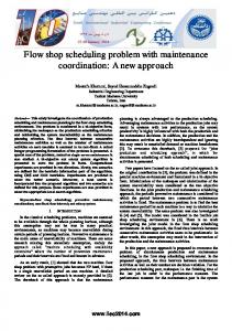
It is interesting to see the variation of the makespan values when the percentage of the affected tasks increases (see Figure 2) or when the δ increases (see Figure 3). In these figures, the vertical left axis represents the makespan scale in hours and the vertical right axis the cpu time scale in seconds. In Figure 2, δ = 10 and remains fixed. The percentage of perturbated tasks goes from 0 to 100%. The best makespan value obtained by the robust GA oscillates between 225 and 260 hours. The figure does not show any link between this value and the percentage of perturbated tasks. The interesting point here is that when the percentage of the perturbated tasks increases, the difference between the expected makespan and the makespan computed in a post-analysis phase remains almost the same. This means that the Robust GA method is reliable for our case study. Some differences can be observed for the CPU time. If we consider this problem at a tactical level, these variations are not so important. In Figure 3, the percentage of perturbated tasks pp is equal to 30%. The value of δ belongs to the range [0, 30] (in hours). Similar conslusions can be drawn from the curves. It seems that there is a linear relation between the M. Sevaux, Y. Le Quéré

13


420 Best makespan e-Makespan p-Makespan CPU time (right axis)

400

1400

380

1200

360

800 320 300

600

Cpu time (in sec.)

Makespan value

1000 340

280 400 260 200 240 220

0 0

20

40 60 Percentage of perturbated tasks

80

100

Figure 2: Variation of the makespan when pp increases 420 Best makespan e-Makespan p-Makespan CPU time (right axis)

400

1400

380

1200

360 340 800 320 300

600

Cpu time (in sec.)

Makespan value

1000

280 400 260 200 240 220

0 0

5

10

15 Value of delta

20

25

30

Figure 3: Variation of the makespan when δ increases M. Sevaux, Y. Le Quéré

14


value of δ and the expected and post-analysis makespan when δ ≥ 5. Again, the difference between these two values remains constant when δ increases.

6

Conclusion

This work is very interesting for the SNCF since we are able to give robust solutions. The Robust GA provides solutions with the same quality the best GA can offer. Moreover, when hazards occurs, it is easy to see that the robust method is the only one able to predict the makespan value with reliability. This method can be easily extended to different types of hazards ( e.g. lateness in at delivery). Another strong point is that any knid of TGVs with different aggregated tasks can be handle with the same method. The work of the decision maker can be simplified. The last step is to use these results for the real application. This is not an easy purpose since all the modifications given by the decision maker should be accepted by the trade unions, otherwise a strike is all what we can expect. This should be done in a wider modification phase of the decision centers at the EIMM factory. Our next work will be to see how this robust GA can be enhanced. The first research axis will be to compute the statistical law of the makespan if for example the processing times follow a normal distribution with known parameters. The current robust evaluation function which is a sampling method, will be replaced by a simple evaluation. This new function will be easy to compute and quicker results will be given by the same method.

References J. Blazewicz, J.K. Lenstra, and A.H.G. Rinnoy Kan, 1983. Scheduling projects subject to resource constraints: classification and complexity. Discrete Applied Mathematics, 5:11–24. J. Branke, 1998. Creating robust solutions by means of evolutionary algo-

M. Sevaux, Y. Le Quéré

15


rithms. In Parallel Problem Solving from Nature V, LNCS vol. 1498, pages 119–128. Springer Verlag, 1998. J. Branke, 2001. Reducing the sampling variance when searching for robust solutions. In L. Spector et al., editor, GECCO 2001 - Proceedings of the Genetic and Evolutionary Computation Conference, pages 235–242. Morgan Kaufmann Publishers, 2001. A.J. Davenport and J.C. Beck, 2000. A survey of techniques for scheduling with uncertainty. Unpublished manuscript. D.E. Goldberg, 1989. Genetic Algorithms in search, Optimization and Machine Learning. Addison Wesley. W. Herroelen and R. Leus, 2002. Project scheduling under uncertainty – survey and research potentials. Invited paper to be published in the special issue of EJOR containing selected papers from PMS2002. J.H. Holland, 1975. Adaptation in natural and artificial systems. Technical report, University of Michigan, Ann Arbor. M.T. Jensen, October 2001. Robust and flexible scheduling with evolutionary computation. PhD thesis, University of Aarhus, Dept. of Computer Science, Denmark. Y. Le Quéré, M. Sevaux, D. Trentesaux, and C. Tahon, Feb. 20–22 2002. Résolution d’un problème industriel de maintenance des tgv a` la sncf. In 4ième conférence nationale de la société fran¸caise de recherche opérationnelle, ROADEF’2002, Paris, France. M-C. Portmann, 1996. Genetic algorithm and scheduling: a state of the art and some propositions. In Proceedings of the workshop on production planning and control, pages I–XIV, Mons, Belgium. Y. Le Quéré, M. Sevaux, D. Trentesaux, and C. Tahon, November, 7-8 2001. Planification réactive des opérations de maintien et d’actualisation réglementaire et technologique des systèmes complexes. In Proceedings M. Sevaux, Y. Le Quéré

16


of the International Conference on Computer aided Maintenance, pages A15/1–12, ENIM, Rabat, Morocco. C.R. Reeves, editor, 1993. Modern heuristic techniques for combinatorial problems. John Wiley & Sons, inc., New York, NY, USA. C.R. Reeves, 1995. A genetic algorithm for flowshop sequencing. Computers and Operations Research, 22(1):5–13. C.R. Reeves, 1997. Genetic algorithms for the operations researcher. Informs Journal on Computing, 9(3):231–250. M. Sevaux and K. Sörensen, 2003. A genetic algorithm for robust schedules in a just- in-time environment. Technical Report LAMIH/SP-2003-1, University of Valenciennes, France. Submitted. K. Sörensen, 2001. Tabu searching for robust solutions. In Proceedings of the 4th Metaheuristics International Conference, pages 707–712, Porto, Portugal. S. Tsutsui, 1999. A comparative study on the effects of adding perturbations to phenotypic parameters in genetic algorithms with a robust solution searching scheme. In Proceedings of the 1999 IEEE Systems, Man, and Cybernetics Conference (SMC’99 Tokyo), pages III–585–591, 1999. S. Tsutsui and A. Ghosh, 1997. Genetic algorithms with a robust solution searching scheme. IEEE Transactions on Evolutionary Computation, 1: 201–208. S. Tsutsui, A. Ghosh, and Y. Fujimoto, 1996. A robust solution searching scheme in genetic search. In H.-M. Voigt, W. Ebeling, I. Rechenberg, and H.-P. Schwefel, editors, Parallel problem solving from nature - PPSN IV, volume 10, pages 543–552, Berlin. Springer. S. Tsutsui and J.C. Jain, 1998. Properties of robust solution searching in multi- dimensional space with genetic algorithms. In Proceedings of the 2nd International Conference on Knowledge-Based Electronic Systems (KES98), 1998. M. Sevaux, Y. Le Quéré

17