Additional Key Words and Phrases: Convex programs, random walks, ... Dimitris Bertsimas was partially supported by the MIT-Singapore alliance. ...... programming,â Research Report 81-39, New York University, Graduate School of Business.
Solving Convex Programs by Random Walks DIMITRIS BERTSIMAS and SANTOSH VEMPALA M.I.T. Minimizing a convex function over a convex set in n-dimensional space is a basic, general problem with many interesting special cases. Here, we present a simple new algorithm for convex optimization based on sampling by a random walk. It extends naturally to minimizing quasi-convex functions and to other generalizations. Categories and Subject Descriptors: F2 [Theory of Computation]: Analysis of Algorithms and Problem Complexity; G3 [Mathematics of Computing]: Stochastic Processes General Terms: Algorithms, Theory Additional Key Words and Phrases: Convex programs, random walks, polynomial time
1. INTRODUCTION The problem of minimizing a convex function over a convex set in Rn is a common generalization of well-known geometric optimization problems such as linear programming as well as a variety of combinatorial optimization problems including matchings, flows and matroid intersection, all of which have polynomial-time algorithms. As such, it represents a frontier of polynomial-time solvability and occupies a central place in the theory of algorithms. In his groundbreaking work, Khachiyan [1979] showed that the Ellipsoid method [Yudin and Nemirovski 1976] solves linear programs in polynomial time. Subsequently, Karp and Papadimitriou [1982], Padberg and Rao [1981], and Gr¨ otschel, Lov´asz and Schrijver [Gr¨ otschel et al. 1981] independently discovered the wide applicability of the Ellipsoid method to combinatorial optimization problems. This culminated in the book by the last set of authors [Gr¨ otschel et al. 1988], in which it is shown that the Ellipsoid method solves the problem of minimizing a convex function over a convex set in Rn specified by a separation oracle, i.e., a procedure which given a point x either reports that the set contains x or returns a halfspace that separates the set from x. For the special case of linear programming, the oracle simply checks if the query point satisfies all the constraints of the linear program, and if not, reports a violated constraint; another well-known special case is semidefinite programming. Vaidya improved the complexity via a more sophisticated Authors’ address: D. Bertsimas, Sloan School of Management and Operations Research Center, M.I.T. and Santosh Vempala, Mathematics Department, M.I.T., Cambridge, MA 02139. Email: {dbertsim, vempala}@mit.edu Dimitris Bertsimas was partially supported by the MIT-Singapore alliance. Santosh Vempala was supported by NSF CAREER award CCR-9875024 and a Sloan foundation fellowship. Permission to make digital/hard copy of all or part of this material without fee for personal or classroom use provided that the copies are not made or distributed for profit or commercial advantage, the ACM copyright/server notice, the title of the publication, and its date appear, and notice is given that copying is by permission of the ACM, Inc. To copy otherwise, to republish, to post on servers, or to redistribute to lists requires prior specific permission and/or a fee. c 20YY ACM 0004-5411/20YY/0100-0001 $5.00
Journal of the ACM, Vol. V, No. N, Month 20YY, Pages 1–0??.
2
·
Bertsimas and Vempala
algorithm [Vaidya 1996]. In this paper, we present a simple new algorithm for the problem, based on random sampling. Its complexity is optimal in terms of the number of oracle queries, but the overall running time can be higher than that of previous algorithms (see Table 1 at the end of Section 2 for a precise comparison). The key component of the algorithm is sampling a convex set by a random walk. Random walks have long been studied for their mathematical appeal, but of late they have also played a crucial role in the discovery of polynomial-time algorithms. Notable applications include estimating the volume of a convex set [Dyer et al. 1991] and computing the permanent of a non-negative matrix [Jerrum et al. 2001]. They have also been used in machine learning and online algorithms [Kalai and Vempala 2002]. Our algorithm is a novel application of random walks to the field of optimization. For the analysis, we prove a generalization of Grunbaum’s theorem [Grunbaum 1960] about cutting convex sets (see Section 4.1); this might be of interest in other settings. So far, we have assumed that the convex set of interest has an efficient separation oracle. A natural question is whether optimization can be solved using a significantly weaker oracle, namely a membership oracle (which reports whether a query point is in the set or not, but provides no other information). One of the main results in [Gr¨ otschel et al. 1988] is that a linear function can be optimized over a convex set K given only by a membership oracle, provided K is “centered”, i.e., we are also given a point y and a guarantee that a ball of some radius r around y is contained in K. The algorithm is intricate and involves a sophisticated variant of the Ellipsoid method, called the shallow-cut Ellipsoid (note that feasibility is trivial since we are given a feasible point). Our algorithm provides a simple solution to this problem. In fact, as we show in Section 6, it solves the following generalization: let K be the intersection of two convex sets K1 and K2 , where K1 is a “centered” convex set with a membership oracle and K2 is a convex set with a separation oracle; find a point in K if one exists. The generalization includes the special case of minimizing a quasi-convex function over a centered convex set given by a membership oracle. This problem (and its special case mentioned above) are not known to be solvable using the Ellipsoid method or Vaidya’s algorithm. 2. THE ALGORITHM In this section, we present an algorithm for the feasibility problem: find a point in a given convex set specified by a separation oracle. This can be used to minimize any quasi-convex function. A function f : Rn → R is called quasi-convex if for any real number t, the set {x ∈ Rn | f (x) ≤ t} is convex. Note that any convex function is also quasi-convex. The problem of minimizing a quasi-convex function is easily reduced to the feasibility problem: to minimize a quasi-convex function f (x) we simply add the constraint f (x) ≤ t and search (in a binary fashion) for the optimal t. In the description below, we assume that the convex set K is contained in the axis-aligned cube of width R centered at the origin; further if K is non-empty then it contains a cube of width r (see e.g. [Bertsimas and Tsitsiklis 1997; Gr¨ otschel et al. 1988] for a justification). The choice of cubes here is somewhat arbitrary; we Journal of the ACM, Vol. V, No. N, Month 20YY.
Solving Convex Programs by Random Walks
·
3
could instead use balls, for example. The parameter L is equal to log Rr . Algorithm. Input: A separation oracle for a convex set K and a number L. Output: A point in K or a guarantee that K is empty. 1. Let P be the axis-aligned cube of width R with center z = 0. 2. Check if z is in K. If so then report z and stop. If not, then let aT x ≤ b be the halfspace containing K reported by the oracle. Set H = {x | aT x ≤ aT z}. 3. Set P = P ∩ H. Pick N random points y1 , y2 , . . . , yN from P . PN Set z to be their average: z = N1 i=1 yi . 4. Repeat steps 2 and 3 at most 2nL times. Report K is empty. Roughly speaking, the algorithm is computing an approximate centroid in each iteration1 . The number of samples required in each iteration, N , is O(n) for an arbitrary convex set in Rn and O(log2 m) if K is a polyhedron with m inequalities (i.e., a linear program). H
K
Z
P
Fig. 1.
An illustration of the algorithm.
The idea behind the algorithm is that the volume of the enclosing polytope P is likely to drop by a constant factor in each iteration. We prove this in Section 4.2 (see Lemma 5) and derive as a consequence that if the algorithm does not stop in 1 The
idea of an algorithm based on computing the exact centroid was suggested in 1965 by Y. Levin [Levin 1965], but is computationally intractable. Journal of the ACM, Vol. V, No. N, Month 20YY.
4
·
Bertsimas and Vempala
Algorithm Ellipsoid Vaidya’s Random walk
Optimization/Feasibility with a Separation oracle
Optimization with a Membership oracle
O(n2 LT + n4 L) O(nLT + n3.38 L) O(nLT + n7 L)
O(n10 LT + n12 L) N/A O(n5 LT + n7 L)
Table I.
Complexity comparison
2nL iterations, then K must be empty with high probability (Theorem 6). Thus, the total number of calls to the separation oracle is at most 2nL. This matches the (asymptotic) bound for Vaidya’s algorithm, and is in general the best possible [Yudin and Nemirovski 1976]. The Ellipsoid algorithm, in contrast, takes O(n2 L) iterations and as many calls to the oracle. Each iteration of our algorithm uses random samples from the current polytope P . The time per iteration depends on how quickly we can draw random samples from P . The problem of sampling from a convex set has received much attention in recent years [Dyer et al. 1991; Lov´asz and Simonovits 1993; Kannan et al. 1997; Lov´asz 1998; Kannan and Lov´asz 1999], in part because it is the only known way of efficiently estimating the volume of a convex set. The general idea is to take a random walk in the set. There are many ways to walk randomly; of these, the ball walk (go to a random point within a small distance) [Kannan and Lov´asz 1999] and hit-and-run (go to a random point along a random direction) [Lov´asz 1998] have the best known bounds on the number of steps needed to draw a random sample. The bounds on the number of steps depend on how “round” the convex set is. For a set that is close to isotropic position (see Section 4), O(n3 ) steps are enough to get one nearly random point from a “good” starting distibution. In our case, the initial convex set, the cube, is indeed in isotropic position. However this might not be the case after some iterations. As we describe in Section 5, this problem can be tackled by computing an affine transformation that keeps the current polytope P in near-isotropic position. We also propose an alternative (in Section 5.1) that avoids this computation and instead incorporates the information about isotropy implicitly in the steps of a random walk by maintaining a set of points. The time per iteration of the algorithm is bounded by O(n4 ) steps of a random walk. Each step of the walk takes O(n2 ) arithmetic operations to implement, and hence the algorithm takes O(n6 ) arithmetic operations per iteration in addition to one oracle call. In Section 6, we describe a variant of the algorithm for optimization when we are given a membership oracle. We conclude this section with a comparison of the complexities of the three algorithms given a separation oracle or given a membership oracle. The parameter T denotes the time taken by the relevant oracle to answer a query. In practice, drawing random samples from convex sets might be much faster than the known worst-case bounds; also, sampling convex sets is an active research area and there might well be faster sampling methods in the future which would directly improve the complexity of the random walk algorithm. Journal of the ACM, Vol. V, No. N, Month 20YY.
Solving Convex Programs by Random Walks
·
5
3. PRELIMINARIES The following definitions will be useful throughout the analysis. We assume that all our convex sets are closed and bounded. Definition 1. A convex set K in Rn is said to be in isotropic position if its center of gravity is the origin, i.e., for a random point x in K, EK (x) = 0 and its covariance matrix is the identity, i.e., EK (xxT ) = I. Equivalently, for any unit vector v (||v|| = 1), Z 1 (v T x)2 dx = 1. vol(K) K In other words, for a set K in isotropic position, the average squared length in any direction is 1. In particular, this implies that Z 1 ||x||2 dx = n. vol(K) K For any full-dimensional convex set, there exists an affine transformation that puts the set in isotropic position. To bring a convex set K with center of gravity z into isotropic position, let A = EK ((x − z)(x − z)T ) be its covariance matrix. Since K is full-dimensional, A is positive definite, and so there exists a matrix B such that B 2 = A−1 . Now define the transformation K ′ = {y : y = B(x − z), x ∈ K}. Then EK ′ (y) = 0 and EK ′ (yy T ) = I. Definition 2. We say that a convex set K is in near-isotropic position if for any unit vector v, Z 1 3 1 ≤ (v T (x − x¯))2 dx ≤ 2 vol(K) K 2
where x ¯ is the centroid of K. Equivalently, the covariance matrix of the uniform distribution over K has eigenvalues between 21 and 32 . The Minkowski sum of two sets A, B in Rn is defined as A + B = {y + z | y ∈ A, z ∈ B}.
For example, the Minkowski sum, x + rB, of a point x and a ball rB of radius r is the ball of radius r centered at x. The following theorem is known as the Brunn-Minkowski inequality (see e.g. [Gardner 2002; Schneider 1993]). Theorem 1. Let A and B be full-dimensional convex subsets of Rn . Then for any λ ∈ [0, 1], 1
1
1
vol(λA + (1 − λ)B) n ≥ λvol(A) n + (1 − λ)vol(B) n . Some of our proofs utilize logconcave functions which we introduce next. Journal of the ACM, Vol. V, No. N, Month 20YY.
6
·
Bertsimas and Vempala
Definition 3. A function f : Rn → R+ is logconcave iff for any two points a, b ∈ Rn and any λ ∈ (0, 1), f (λa + (1 − λ)b) ≥ f (a)λ f (b)1−λ . In other words, a nonnegative function f is logconcave if its support is convex and log f is concave. For example, a function that is constant over a bounded convex set and zero outside the set is logconcave. Another example is a Gaussian density function. It can be easily verified from the definition above that the product of two logconcave functions is also logconcave (but their sum is not). Finally, we will use the following simple fact from linear algebra. When we apply a linear transformation A to a compact convex set K, then the volume of the resulting set AK is |det(A)|vol(K). 4. ANALYSIS In this section, we prove that with high probability, the algorithm needs only O(n) random points per iteration and O(nL) iterations. Section 5 describes how to efficiently obtain the random points in each iteration. 4.1 Geometric properties The following theorem was proved by Grunbaum. Theorem 2. [Grunbaum 1960] For a convex set K in Rn , any halfspace that contains the centroid of K also contains at least 1/e of the volume of K. Here, we prove a generalization. Theorem 3. Let K be a convex set in isotropic position and z be a point at distance t from its centroid. Then any halfspace containing z also contains at least 1 e − t of the volume of K. Theorem 3 with t = 0 clearly implies Grunbaum’s theorem for isotropic convex sets. Further, any convex set K can be mapped to an isotropic one by an affine transformation which changes the volume of any subset by the same factor; so the ratio of two volume remains unchanged, and in particular for any halfspace H, the ratio vol(H ∩ K)/vol(K) is preserved under an affine transformation. Thus Grunbaum’s theorem is implied in general. The proof of Theorem 3 will rely on the next lemma. The function defined in the lemma is the distribution induced by cross-sectional areas perpendicular to some vector a. Lemma 4. For an isotropic convex set K and any unit vector a ∈ Rn , define a function f : R → R+ as Z 1 dx. f (y) = vol(K) x∈K,aT x=y Then max f (y) < 1. y∈R
Journal of the ACM, Vol. V, No. N, Month 20YY.
Solving Convex Programs by Random Walks
·
7
Proof. Fix a unit vector a ∈ Rn . Let fK be the one-dimensional marginal distribution Z 1 dx. fK (y) = vol(K) x∈K,aT x=y In other words, fK (y) is the (n − 1)-dimensional volume of K intersected with the hyperplane aT x = y, as a fraction of the volume of K. Define Z Z yfK (y) dy and I(K) = (y − y¯K )2 fK (y)dy. y¯K = R
R
Note that I(K) is the variance (or moment of inertia) of K along the vector a. By translating K, we can assume without loss of generality that y¯K = 0. Further, by a rotation, we can assume that a = (1, 0, . . . , 0), i.e., the unit vector along x1 . We will, in fact, prove a slightly stronger statement: for any convex body K for which fK is defined as above and which satisfies Z Z y 2 fK (y) dy = 1, (1) yfK (y) dy = 0 and R
R
we have maxR fK (y) < 1. To this end, let K be a convex body satisfying (1) for which max fK (y) is the maximum possible. We will show that K can be assumed to be an isotropic cone. To see this, first consider the set K ′ obtained by replacing each cross-section K ∩ {x|x1 = y} by an (n − 1)-dimensional ball of area fK (y) and centered at the point (y, 0, . . . , 0). Clearly, the set K ′ has the same volume as K. Further, if we let r(y) denote the radius of the (n − 1)-dimensional ball at y, then r is a concave function. This follows from the Brunn-Minkowski inequality (Theorem 1): Let A1 be the cross-section at y1 , A2 the cross-section at y2 and A the cross-section at λy1 + (1 − λ)y2 for some λ ∈ [0, 1]. Then, 1
1
1
1
vol(A) n−1 ≥ vol(λA1 + (1 − λ)A2 ) n−1 ≥ λvol(A1 ) n−1 + (1 − λ)vol(A2 ) n−1 . This implies that r(λy1 +(1−λ)y2 ) ≥ λr(y1 )+(1−λ)r(y2 ), i.e., r is concave. Hence the set K ′ is convex. Further, fK ′ = fK and so (1) continues to be satisfied. So, without loss of generality, we can assume that K is symmetric about the x1 axis. If K is a cone, we are done. If not, let y ∗ be a point where fK is maximum and suppose that y ∗ ≥ 0 (the other case is symmetric). Divide K into three parts: K1 = K ∩ {x|x1 ≤ 0},
K2 = K ∩ {x|0 ≤ x1 ≤ y ∗ },
K3 = K ∩ {x|x1 ≥ y ∗ }.
We will now use the following claim to simplify K (which essentially says that moving mass away from the center of gravity can only increase the moment of inertia). Claim. Suppose a set C ′ is obtained from a set C by moving mass away from the centroid of C or keeping it at the same distance along the x1 axis, i.e., for any t ≥ 0, vol(C ′ ∩ {x : |x1 | ≥ t}) ≥ vol(C ∩ {x : |x1 | ≥ t}). Then I(C ′ ) ≥ I(C). To prove the claim, assume that the centroid of C is 0. Let the coordinate of a point x change from x1 to x1 + g(x) where g(x) is a real number with the same Journal of the ACM, Vol. V, No. N, Month 20YY.
8
·
Bertsimas and Vempala
K2 K2’
K
K1
Fig. 2.
K3
K1’
K3’
a
The proof of Lemma 4.
sign as x1 . Note that EC (x1 ) = 0 by assumption. I(C ′ ) = VarC ′ (x1 ) = VarC (x1 + g(x)) = EC ((x1 + g(x))2 ) − EC (x1 + g(x))2 = VarC (x1 ) + VarC (g(x)) + 2EC (x1 g(x)) ≥ I(C) since x1 g(x) ≥ 0 for every point x. We now make the following changes to our set K. Replace K1 by a cone K1′ of the same volume with base area equal to fK (0). Replace K2 by a truncated cone K2′ of height y ∗ , top area fK (0) and base area fK (y ∗ ). Finally replace K3 by a cone K3′ of base area fK (y ∗ ) and vol(K3′ ) = vol(K3 ) + vol(K2 ) − vol(K2′ ). Let K ′ = K1′ ∪ K2′ ∪ K3′ be the new convex set. See Figure 2 for an illustration. During the first step, by the claim, the moment of inertia can only increase. After the first step, the new center of gravity along the x1 axis can only have moved to the left (since mass moves to the left). Thus the next two steps also move mass away from the center of gravity, and we can apply the claim. At the end, we get I(K ′ ) ≥ I(K),
vol(K) = vol(K ′ ),
max fK (y) = max fK ′ (y).
If I(K ′ ) > I(K), then we can scale down K ′ along the x1 axis and scale it up perpendicular to the x1 axis, in such a way as to maintain the volume, achieve I(K ′ ) = I(K), and have max fK ′ (y) > max fK (y). This is a contradiction. Thus, we can assume that K has the form of K ′ , i.e., Ki = Ki′ . At this point, one could perform a somewhat tedious (but routine) computation to show that a cone of the same volume as K and base area fK (y ∗ ) has a larger moment of inertia than K, leading to the same contradiction unless K itself is a cone. The following observation, again using the claim, avoids this computation. For a point y ∈ [0, y ∗ ] along the x1 axis, consider the subsets S1 = {x|x1 ≤ −y}, S2 = {x| − y ≤ Journal of the ACM, Vol. V, No. N, Month 20YY.
Solving Convex Programs by Random Walks
y
·
9
y
0
Fig. 3.
The proof of Lemma 4 continued.
x1 ≤ y} and S3 = {x|x1 ≥ y}. Now leave the set S3 unchanged, replace the set S2 by the truncated cone S2′ with base area fK (y) and top area fK (−y) and the set S1 by the cone S1′ with base area fK (−y) and volume vol(K) − vol(S3 ) − vol(S2′ ), so that the total volume is unchanged. This is illustrated in Figure 3. If K1 ∪K2 is not a cone, then there is some y > 0 for which we can do the above replacement. But then, by construction, we are moving mass away from the center (mass at distance at most y along the x1 axis is moved to distance at least y), and so by the claim, the moment of inertia can only go up. Hence, we can assume that K1 ∪ K2 is a cone of base area fK (y ∗ ) and thus K is the union of two cones with the same base. Now it is straightforward to check that a cone of the same volume as K and base area fK (y ∗ ) has a larger moment of inertia, and so K itself must be a cone. q Finally, an isotropic cone has height h = n + 1 n+2 n and volume Ah/n where A is the area of the base. Hence, n n A = = max fK (y) = Ah/n h n+1
r
n . n+2
Using the lemma, we can prove Theorem 3.
Proof. (of Theorem 3) Let K be a convex set in isotropic position and let z be a point at distance t from its centroid. Consider a hyperplane through z with normal vector a such that ||a|| = 1. Let f be defined as in Lemma 4. By the Lemma, maxy∈R f (y) < 1. Without loss of generality, assume that aT z ≥ 0. The Journal of the ACM, Vol. V, No. N, Month 20YY.
10
·
Bertsimas and Vempala
fraction of the volume of K that is cut off by the halfspace aT x ≥ aT z is at least Z ∞ Z ∞ Z aT z f (y)dy = f (y)dy − f (y)dy aT z
0
0
aT z
1 − f (y)dy (using Theorem 2) e 0 1 ≥ − |aT z| (using Lemma 4) e 1 1 ≥ − ||z|| = − t. e e ≥
Z
4.2 Number of iterations The next theorem, whose proof uses Theorem 3, is the key to bounding the number of iterations. In this section, by high probability we mean probability higher than any fixed constant. Lemma 5. The volume of P drops by a factor of iteration.
2 3
with high probability in each
Proof. We will prove that for any convex set K, if z is the average of sufficiently many random samples from K, then any halfspace through z cuts off a constant fraction of the volume of K. To this end we can assume without loss of generality that K is in isotropic position. This is because of two facts: (i) as shown earlier, any convex set can be brought into isotropic position by an affine transformation and (ii) on applying an affine transformation A to K, the volume scales by det(A), i.e., vol(AK) = |det(A)|vol(K); so affine transformations preserve ratios of volumes. Let y1 , y2 , . . . , yN be the N samples drawn uniformly from K. Let
Then, using the isotropy of K, E(yi ) = 0
N 1 X yi . z= N i=1
and
E(||yi ||2 ) = n.
Thus, n . N n by choosing N = O(n) we can have ||z|| smaller than any Since E(||z||2 ) = N constant. By Theorem 3 any halfspace aT x ≥ aT z passing through z cuts off at least 1e − ||z|| fraction of the volume of K. We choose N so that 1e − ||z|| ≥ 31 with high probability. Then any halfspace through z cuts off at least 13 of the volume of K. E(z) = 0
and
E(||z||2 ) =
We remark that in the proof above we only need the random samples to be pairwise independent. This is because the only quantity we needed to bound was the distance of z from the origin for an isotropic convex set, and for this we only used the variance of ||z||. The bounds for the variance only need pairwise independence. Journal of the ACM, Vol. V, No. N, Month 20YY.
Solving Convex Programs by Random Walks
·
11
Theorem 6. If the algorithm does not find a feasible point in 2nL iterations, then with high probability, the given convex set is empty. Proof. The initial volume of P is Rn . If the set K is nonempty, then it has volume at least rn . Thus the number of iterations in which the volume drops by 2/3 is at most � n� R R = n log 23 log 23 n r r and thus with high probability, the total number of iterations is at most 2nL. 4.3 A better bound for linear programming For the case of linear programming, when the target convex set K is a polyhedron defined by m linear inequalities, a smaller number of samples can be used in each iteration. The next lemma proves that any single violated inequality is detected with high probability. The main idea is that since the separation oracle will simply return one of only m hyperplanes in case of a violation, one can apply the “union bound” to show that with high probability a small sample will detect a violation. This is in contrast to the general case where the separation oracle might return one of infinitely many possibilities. Lemma 7. Let K be a convex set and z be the average of N random samples from K. Let a be a fixed unit vector. Then the √probability that the halfspace aT x ≤ aT z cuts off at least 31 of K is at least 1 − 2−c N for some constant c.
Proof. Assume without loss of generality that P is in isotropic position. Let Yi = aT yi for i = 1, . . . , N . Then, Yi ’s are independent random variables with distribution given by the logconcave function Z 1 dx. f (y) = vol(K) x∈K,aT x=y We have E(Yi ) = 0
and
E(Yi2 ) = 1.
Let Z = aT z = Then,
N 1 X Yi . N i=1
1 . N Now the distribution of Z is the convolution of the distributions of the Yi ’s and is also logconcave [Prekopa 1973]. Thus, there is a constant D such that for any t ≥ 1, � � t P |Z| > √ ≤ e−Dt . N As a consequence, for N > 1/c2 , E(Z) = 0
and
E(Z 2 ) =
P r(|aT z| > c) ≤ e−cD
√ N
.
Journal of the ACM, Vol. V, No. N, Month 20YY.
12
·
Bertsimas and Vempala
By choosing c small enough, we get that the halfspace aT x ≤ aT z cuts off at least 31 √ ′ of the volume of P with probability at least 1 − e−c N for some absolute constant c′ . Corollary 8. Let the target convex set be the intersection of m halfspaces. Then with N = O(log2 m), the volume of P drops by a factor of 23 in each iteration with high probability. Proof. As in the proof of Lemma 5, let y1 , . . . , yN be random variables denoting the samples from the current polytope P and let z be their average. In Lemma 5, we showed that for any unit vector a, the hyperplane normal to a and passing through z is likely to cut off at least 31 of the volume of P . Suppose that the target set K is the intersection of m halfspaces defined by hyperplanes with normal vectors a1 , . . . , am (with ||ai || = 1). Then we only need to show that each of the hyperplanes aTi x = aTi z cuts off at least 13 of P . This is because the separation oracle for the target convex set (which simply checks the m halfspaces and reports one that is violated) will return a hyperplane parallel to one of these. By Lemma 7, any single halfspace aT x ≤ aT z cuts off 31 of P with probability √ at least 1 − 2−c N for some constant c. Setting N = O(log2 m) implies that with high probability any one of m halfspaces will cut off a constant fraction of P . 5. SAMPLING AND ISOTROPY In each iteration, we need to sample the current polytope. For this we take a random walk. There are many ways to walk randomly but the two ways with the best bounds on the mixing time are the ball walk and hit-and-run. They are both easy to describe. Ball walk (1) Choose y uniformly at random from the ball of radius δ centered at the current point x. (2) If y is in the convex set then move to y; if not, try again. Hit-and-run (1) Choose a line ℓ through the current point x uniformly at random. (2) Move to a point y chosen uniformly from K ∩ ℓ. The mixing time of the walk depends on how close the convex set is to being in isotropic position (recall definition 2). In addition to isotropy, the starting point (or distribution) of a random walk plays a role in the bounds on the mixing time. The best bounds available are for a warm start – a starting distribution is already close to the stationary distribution π. The total variation distance between two distributions σ and π with support K is defined as: ||σ − π|| = sup |σ(A) − π(A)|. A⊆K
The following result is paraphrased from [Lov´asz 1998]. Theorem 9. [Lov´ asz 1998] Let K be a near-isotropic convex set, σ be any distribution on it with the property that for any set S with π(S) ≤ ǫ, we have σ(S) ≤ 10ǫ. Journal of the ACM, Vol. V, No. N, Month 20YY.
Solving Convex Programs by Random Walks
·
13
3
Then after Ω( nǫ2 log 1ǫ ) steps of hit-and-run starting at σ, the distribution obtained has total variation distance less than ǫ from the uniform distribution. A similar statement holds for ball walk with step size δ = Θ( √1n ) (see [Kannan and Lov´asz 1999]). One advantage of hit-and-run is that there is no need to choose the “step size” δ. The problem with applying this directly in our algorithm to the current polytope P is that after some iterations P may not be in near-isotropic position. One way to maintain isotropic position is by using random samples to calculate an affine transformation. It was proven in [Kannan et al. 1997] that for any convex set, O(n2 ) samples allow us to find an affine transformation that brings the set into near-isotropic position. This was subsequently improved to O(n log2 n) [Rudelson 1999]. The procedure for a general convex set K is straightforward: (1) Let y1 , y2 , . . . , yN be random samples from K. (2) Compute y¯ =
N 1 X yi N i=1
and
Y =
N 1 X (yi − y¯)(yi − y¯)T . N i=1
(2)
The analysis of this procedure rests on the following consequence of a more general lemma due to Rudelson [Rudelson 1999]. Lemma 10. [Rudelson 1999] Let K be a convex body in Rn in isotropic position and η > 0. Let y1 , . . . , yN be independent random points uniformly distributed in K, with np n N ≥ c 2 log 2 max{p, log n}. η η where c is a fixed absolute constant and p is any positive integer. Then p ! N 1 X T ≤ ηp yi yi − I E N i=1
Corollary 11. Let K be a convex set and y¯ and Y be defined as in (2). There is an absolute constant c such that for any integer p ≥ 1, and N ≥ cpn log n max{p, log n}, 1 with probability at least 1 − 2p−1 , the set 1
K ′ = {x|Y 2 x + y¯ ∈ K} is in near-isotropic position. Proof. Without loss of generality, we can assume that K is in isotropic position. Let Y0 = Then applying Lemma 10 we have
N 1 X yi yiT . N i=1
E(||Y0 − I||p ) ≤ η p . Journal of the ACM, Vol. V, No. N, Month 20YY.
14
·
Bertsimas and Vempala
Hence, P r(||Y0 − I|| > 2η) = P r(||Y0 − I||p > (2η)p ) E[||Y0 − I||p ] ≤ (2η)p 1 ≤ p 2 Now Y = Y0 − y¯y¯T , and so ||Y − I|| ≤ ||Y0 − I|| + ||¯ y ||2 . The random variable y¯ 2 has a logconcave distribution and E(||¯ y || ) = n/N . So, there is a constant D such that for any t ≥ 1, r � � n P r ||¯ y || > t ≤ e−Dt . N p Using η = 1/8 and t = N/4n, we get that with N ≥ cpn log n max{p, log n} points (this is a different constant c from that in Lemma 10), � � 1 1 ≤ p−1 . P r ||Y − I|| > 2 2 Next we evaluate max v T Y v and min v T Y v over unit vectors v. v T Y v = v T Iv + v T (Y − I)v ≤ 1 + ||Y − I||. v T Y v = v T Iv + v T (Y − I)v ≥ 1 − ||Y − I||. 1 , v T Y v is between Thus with probability 1 − 2p−1 ′ and so K is in near-isotropic position.
1 2
and
3 2
for any unit vector v,
In fact, using N = O∗ (n) points, the probability of failure in each iteration can be made so low (inverse polynomial) that the probability of failure over the entire course of the algorithm is smaller than any fixed constant. In order to keep the sampling efficient, we calculate such an affine transformation in each iteration, using samples from the previous iteration. However, we do not need to apply the transformation to the current polytope P . Instead, we could keep P as it is and use the following modified random walk: From a point x, 1
(1) Choose a point y uniformly at random from x + δY 2 Bn . (2) If y is in the convex set then move to y; if not, try again. 1
A similar modification (choose the line ℓ from Y 2 Bn rather than Bn ) can be made to hit-and-run also. In this paper, we do not deal with the technical difficulties caused by near-uniform sampling of nearly-independent points. For a detailed discussion of those issues, the reader is referred to [Kannan et al. 1997]. Theorem 12. Each iteration of the algorithm can be implemented in O∗ (n4 ) steps of a random walk in P . Journal of the ACM, Vol. V, No. N, Month 20YY.
Solving Convex Programs by Random Walks
·
15
Proof. Our initial convex set, the cube, is in isotropic position and it is easy to sample from it. Given a warm start in a current polytope P in near-isotropic position, we take O∗ (n3 N ) steps of a random walk to get 2N nearly random samples (using Theorem 9). We compute the average z of N of these, and if z is not in the target convex set, then we refine P with a new halfspace H to get P ′ . Of the remaining N points, at least a constant fraction (say 14 ) are in P ′ with high probability. Further, their distribution is nearly uniform over P ′ . Using these 1 points, we estimate Y 2 by the formula of Corollary 11. With high probability this is a nonsingular matrix. By Corollary 11, we only need N = O∗ (n) samples in each iteration. The reason for discarding the subset of samples used in computing the average is to avoid correlations with future samples. 5.1 An isotropic variant Here we describe an alternative method which implicitly maintains isotropy. It has the advantage of completely avoiding the computation of the linear transformation 1 Y 2. Instead of walking with a single point, consider the following multi-point walk: Maintain m points v1 , v2 , . . . , vm . For each j = 1, . . . , m, Pm (1) Choose a direction ℓ = i=1 αi vi where α1 , . . . , αm are drawn independently from the standard normal distribution. (2) Move vj to a random point in K along ℓ.
Theorem 13. Suppose the multi-point walk is started with m = Ω(n log2 n) points drawn from a distribution σ that satisfies σ(S) ≤ 10ǫ for any subset S with 3 π(S) ≤ ǫ. Then their joint distribution after Ω(m nǫ2 log 1ǫ ) steps has total variation distance less than ǫ from the distribution obtained by picking m random points uniformly and independently from π. Proof. The random walk described above is invariant under affine transformations, meaning there is a one-to-one map betweeen a walk in K and a walk in an affine transformation of K; hence we can assume that K is isotropic. Now consider a slightly different walk where we keep m points, pick one and make a standard hit-and-run step, i.e., the direction is chosen uniformly. The corresponding Markov chain has states for each m-tuple of points from K, and since each point is walking independently, it follows from Theorem 9 that the chain has the bound described above. Compare this to the Markov chain for our random walk. The stationary distribution is the same (our Markov chain is symmetric). The main observation is that for v1 , . . . , vm picked at random and m = Ω(n log2 n), Corollary 11 imples that with high probability, the matrix of inertia has eigenvalues bounded by constants from above and below. We can choose m so that this probability is 1 − n110 . Thus, for all but a n110 fraction of states, the probability of each single transition of our Markov chain is within a constant factor of the first Markov chain. So the conductance of any subset of probability greater than n18 (say) is within a constant factor of its conductance in the first chain. Since we start out with a warm distribution (i.e., a large subset), this implies the bound on the mixing time. Journal of the ACM, Vol. V, No. N, Month 20YY.
16
·
Bertsimas and Vempala
Thus the entire convex programming algorithm now consists of the following: We maintain 2N random points in the current polytope P . We use N of them to generate the query point and refine P . Among the rest, we keep those that remain in P , and continue to walk randomly as described above till we have 2N random points again. 6. A GENERALIZATION In this section, we consider the problem of optimization over a convex set given by a weaker oracle, namely a membership oracle. In [Gr¨ otschel et al. 1988], it is shown that this is indeed possible using a sophisticated variant of the ellipsoid algorithm, provided we have a centered convex set K. That is, in addition to the membership oracle, we are given a point y ∈ K, and a guarantee that a ball of radius r around y is contained in K. The algorithm and proof there are quite nice but intricate2 . Our algorithm provides a solution for a more general problem: K is the intersection of two convex sets K1 and K2 . We are given a separation oracle for K1 , a membership oracle for K2 and a point in K2 . The problem is to minimize a convex function over K. Theorem 14. Let K = K1 ∩K2 where K1 is given by a separation oracle and K2 by a membership oracle. Let R be the radius of an origin-centered ball containing K. Then, given a point y ∈ K2 such that the ball of radius r around y is contained in K2 (i.e., K2 is centered), the optimization problem over K can be solved in time polynomial in n and log Rr . Proof. It is clear that optimization is reducible to feasibility, i.e., we just need to find a point x in K or declare that K is empty. We start with P as K2 intersected with the ball of radius 2R with center y and apply our algorithm. The key procedure, a random walk in P , needs a point in P and a membership oracle for P , both of which we have initially and at each iteration. Using O∗ (n) samples we can bring P into near-isotropic position. Also, each subsequent query point z is guaranteed to be in K2 , since it is the average of points from K2 . Thus, the algorithm needs at most O(n log Rr ) iterations and O(n log Rr ) calls to the separation oracle for K1 . Each iteration (after the first) makes O∗ (n4 ) calls to the membership oracle for K2 . To bring the initial set P into isotropic position, we can adapt the “chain of bodies” procedure of [Kannan et al. 1997]. Since K2 is centered, it contains a ball of radius r around y. Scale up so that y + rBn is in isotropic position and call it Q (just for convenience; this has the effect of scaling up R also). Now consider 1 Q′ = P ∩ (y + 2 n rBn ), i.e., K2 intersected with the ball of radius 21/n r around y. The volume of Q′ is at most twice the volume of Q. This is because 1
1
1
Q′ = P ∩ (y + 2 n rBn ) ⊆ 2 n (P ∩ (y + rBn )) = 2 n Q.
Thus, a uniform sample from Q provides a warm start for sampling from Q′ . Sample from Q′ , drawing each sample in poly(n) time and use the samples to calculate an affine transformation that would put Q′ in isotropic position. Apply the transformation to P . Reset Q to be the transformed Q′ , y to be its center of gravity and r to be the radius of the ball around y containing Q. Again let Q′ be the 2 It
is not known whether Vaidya’s algorithm can be extended to solve this problem.
Journal of the ACM, Vol. V, No. N, Month 20YY.
Solving Convex Programs by Random Walks
·
17
intersection of P with the ball of radius 21/n r around y. After at most O(n log Rr ) such phases, P will be in near-isotropic position. 7. EXTENSIONS The methods of this paper suggest the following interior point algorithm for optimization. Suppose we want to maximize cT x over a full-dimensional convex set K. We start with a feasible solution z1 in K. Then add the constraint cT x ≥ cT z1 and let K := K ∩ {x | cT x ≥ cT z1 }. Next we generate N random points yi in the set K and let z2 be their average. If cT z2 − cT z1 < ǫ we stop; otherwise we set K := K ∩ {x | cT x > cT z2 }, and continue. The algorithms seems to merit empirical evaluation; in practice, it might be possible to sample more efficiently than the known worst-case bounds. The algorithm presents a strong motivation to find geometric random walks that mix faster. Acknowledgement. We thank Adam Kalai, Ravi Kannan, Laci Lov´asz and Mike Sipser for useful discussions and their encouragement. REFERENCES D. Bertsimas and J. Tsitsiklis, Introduction to Linear Optimization, Athena Scientific, 1997. M. Dyer, A. Frieze and R. Kannan, “A random polynomial time algorithm for estimating the volumes of convex bodies,” Journal of the ACM, 38, 1–17, 1991. R. J. Gardner, “The Brunn-Minkowski inequality,” Bulletin of the AMS, 39(3), 355-405, 2002. M. Gr¨ otschel, L. Lov´ asz, and A. Schrijver, “The ellipsoid method and its consequences in combinatorial optimization,” Combinatorica 1, 169–197, 1981. M. Gr¨ otschel, L. Lov´ asz, and A. Schrijver, Geometric Algorithms and Combinatorial Optimization, Springer, 1988. B. Grunbaum, “Partitions of mass-distributions and convex bodies by hyperplanes,” Pacific J. Math. 10, 1257–1261, 1960. M. Jerrum, A. Sinclair, E. Vigoda, “A polynomial-time approximation algorithm for the permanent of a matrix with non-negative entries,” Proc. 33rd Annual ACM STOC, 712–721, 2001. A. Kalai and S. Vempala, “Efficient algorithms for universal portfolios,” J. Machine Learning Research 3, 423–440, 2002. R. Kannan and L. Lov´ asz, “Faster mixing via average conductance,” Proc. 31st Annual ACM STOC, 282–287, 1999. R. Kannan, L. Lov´ asz and M. Simonovits. “Isoperimetric problems for convex bodies and a localization lemma,” Discrete Computational Geometry 13, 541–559, 1995. R. Kannan, L. Lov´ asz and M. Simonovits. “Random walks and and an O ∗ (n5 ) volume algorithm for convex sets,” Random Structures and Algorithms 11, 1–50, 1997. R. Kannan, J. Mount, S. Tayur, “A randomized algorithm to optimize over certain convex sets,” Math. Oper. Res. 20(3), 529–549, 1995. R. M. Karp and C. H. Papadimitriou, “On linear characterization of combinatorial optimization problems,” Siam J. Comp., 11, 620–632, 1982. L. G. Khachiyan, “A polynomial algorithm in linear programming,” (in Russian), Doklady Akedamii Nauk SSSR, 244, 1093–1096, 1979 (English translation: Soviet Mathematics Doklady, 20, 191–194, 1979). A. Yu. Levin, “On an algorithm for the minimization of convex functions,” (in Russian), Doklady Akedemii Nauk SSSR, 160, 1244–1247, 1965 (English translation: Soviet Mathematics Doklady, 6, 286-290, 1965). L. Lov´ asz, “Hit-and-run mixes fast,” Mathematical Programming 86, 443–461, 1998. L. Lov´ asz and M. Simonovits, “Random walks in convex bodies and an improved volume algorithm,” Random Structures and Algorithms 4, 259–412, 1993. Journal of the ACM, Vol. V, No. N, Month 20YY.
18
·
Bertsimas and Vempala
M. W. Padberg and M. R. Rao, “The Russian method for linear programming III: Bounded integer programming,” Research Report 81-39, New York University, Graduate School of Business Administration, New York, 1981. A. Prekopa, “On logarithmic concave measures and functions,” Acta Sci. Math. Szeged, 34, 335– 343, 1973. M. Rudelson, “Random vectors in the isotropic position,” J. Funct. Anal. 164, 60–72, 1999. R. Schneider, Convex Bodies: The Brunn-Minkowski Theory, Cambridge University Press, Cambridge, 1993. P. M. Vaidya, “A new algorithm for minimizing convex functions over convex sets,” Mathematical Programming, 73, 291–341, 1996. D. B. Yudin and A. S. Nemirovski, “Evaluation of the information complexity of mathematical programming problems,” (in Russian), Ekonomika i Matematicheskie Metody 12, 128-142, 1976 (English translation: Matekon 13, 2, 3-45, 1976).
Journal of the ACM, Vol. V, No. N, Month 20YY.