Hindawi Publishing Corporation Journal of Computational Methods in Physics Volume 2014, Article ID 381074, 10 pages http://dx.doi.org/10.1155/2014/381074
Research Article Solving Fractional Diffusion Equation via the Collocation Method Based on Fractional Legendre Functions Muhammed Syam and Mohammed Al-Refai Department of Mathematical Sciences, United Arab Emirates University, Al Ain, UAE Correspondence should be addressed to Muhammed Syam;
[email protected] Received 10 April 2014; Revised 24 June 2014; Accepted 1 July 2014; Published 24 July 2014 Academic Editor: Mikhail Tokar Copyright © 2014 M. Syam and M. Al-Refai. This is an open access article distributed under the Creative Commons Attribution License, which permits unrestricted use, distribution, and reproduction in any medium, provided the original work is properly cited. A formulation of the fractional Legendre functions is constructed to solve the generalized time-fractional diffusion equation. The fractional derivative is described in the Caputo sense. The method is based on the collection Legendre and path following methods. Analysis for the presented method is given and numerical results are presented.
1. Introduction We consider the generalized time-fractional diffusion equation of the form 𝐷𝑡𝛼 𝑢 (𝑥, 𝑡) = 𝑎 (𝑥, 𝑡) 𝐷𝑥2 𝑢 (𝑥, 𝑡) + 𝑓 (𝑥, 𝑡) , 𝑥 ∈ (−1, 1) , 𝑡 ∈ (0, 𝑇) ,
(1)
with initial and boundary conditions 𝑢 (−1, 𝑡) = ℎ1 (𝑡) ,
𝑢 (1, 𝑡) = ℎ2 (𝑡) ,
𝑢 (𝑥, 0) = 𝑔 (𝑥) , (2)
where 𝑎, 𝑓 ∈ 𝐶1 ([−1, 1] × [0, 𝑇]), 𝑔 ∈ 𝐶[−1, 1], ℎ1 , ℎ2 ∈ 𝐶[0, 𝑇], 𝑇 > 0, and 0 < 𝛼 ≤ 1. For 𝛼 = 1, the fractional diffusion equation is reduced to a conventional diffusion-reaction equation which is well studied, so we focus on 0 < 𝛼 < 1. Some existence and uniqueness results of Problem (1)-(2) were established in [1]. In recent years, great interests were devoted to the analytical and numerical treatments of fractional differential equations (FDEs). Usually, FDEs appear as generalizations to existing models with integer derivative and they also present new models for some physical problems [2, 3]. In general, FDEs do not possess exact solutions in closed forms, and, therefore, numerical methods such as the variational iteration (VIM) [4, 5], the homotopy analysis method (HAM) [6, 7], and the Adomian decomposition method (ADM) [8, 9] have
been implemented for several types of FDEs. Also, the maximum principle and the method of lower and upper solutions have been extended to deal with FDEs and obtain analytical and numerical results [10, 11]. The Tau method, the pseudospectral method, and the wavelet method based on the Legendre polynomials have been implemented for several types of FDEs [12–14]. Kazem et al. [12] have constructed the Legendre functions of fractional order and discussed some of their properties. The resulting Legendre function operational and product matrices, together with the Tau method, have been implemented to solve linear and nonlinear fractional differential equations. The effectiveness of the approach has been examined through several examples. In [13], a fractional diffusion equation is considered, where the fractional derivative of order 1 < 𝛼 ≤ 2 refers to the spatial variable 𝑥. The Legendre pseudospectral method is implemented to solve the problem, where the solution is expanded with regular Legendre polynomials. As a result, a system of linear equation has been obtained and integrated using the finite difference method. However, in solving fractional differential equations of order 𝛼 using series expansions, it is common and more efficient to expand the solution with fractional functions of 𝑖𝛼 the form ∑𝑁 𝑖=0 𝑐𝑖 𝑥 . Rawashdeh [14] has implemented the Legendre wavelets method for integrodifferential equations with fractional order. The Legendre collocation method has been implemented for wide classes of differential equations and the effectiveness
2
Journal of Computational Methods in Physics
of the method is illustrated [15]. In the recent work, we intend to apply the collocation method based on the shifted fractional Legendre functions to integrate the Problem (1)-(2). To the best of our knowledge, the method has not been developed to integrate fractional diffusion equations of the form (1)-(2). We organize this paper as follows. In Section 2, we present basic definitions and results of fractional derivative. In Section 3, we present the numerical technique for solving Problem (1)-(2). In Section 4, we present some numerical results to illustrate the efficiency of the presented method. Finally we conclude with some comments in Section 5.
In this section, we present the definition and some preliminary results of the Caputo fractional derivative, as well as the definition of the fractional-order Legendre functions and their properties. Definition 1. A real function 𝑓(𝑡), 𝑡 > 0, is said to be in the space 𝐶𝜇 , 𝜇 ∈ R, if there exists a real number 𝑝 > 𝜇, such that 𝑓(𝑡) = 𝑡𝑝 𝑓1 (𝑡), where 𝑓1 (𝑡) ∈ 𝐶[0, ∞), and it is said to be in the space 𝐶𝜇𝑚 if 𝑓(𝑚) ∈ 𝐶𝜇 , 𝑚 ∈ N. Definition 2. The left Riemann-Liouville fractional integral of order 𝛿 ≥ 0, of a function 𝑓 ∈ 𝐶𝜇 , 𝜇 ≥ −1, is defined by 𝑡 { 1 ∫ (𝑡 − 𝑠)𝛿−1 𝑓 (𝑠) 𝑑𝑠, 𝛿 > 0, 𝐼 𝑓 (𝑡) = { Γ (𝛿) 0 𝛿 = 0. {𝑓 (𝑡) ,
((1 − 𝑥2 ) 𝐿𝑘 (𝑥)) + 𝑘 (𝑘 + 1) 𝐿 𝑘 (𝑥) = 0,
Among the properties of the Legendre polynomials we list the following [19]: 1
0, 𝑖=𝑗̸
(1) ∫−1 𝐿 𝑖 (𝑥)𝐿 𝑗 (𝑥)𝑑𝑥 = (2/(2𝑖+1))𝛿𝑖𝑗 , where 𝛿𝑖𝑗 = {1, 𝑖=𝑗},
(3)
(3) 𝐿 𝑖 (±1) = (±1)𝑖 . In order to use these polynomials on the interval [0, 1], we define the shifted Legendre polynomials by 𝑆𝑖 (𝑥) = 𝐿 𝑖 (2𝑥−1). Using the change of variable 𝑧 = 2𝑥−1, 𝑆𝑖 (𝑥) has the following properties: 1
(1) ∫0 𝑆𝑖 (𝑥)𝑆𝑗 (𝑥)𝑑𝑥 = (1/(2𝑖 + 1))𝛿𝑖𝑗 , (2) 𝑆𝑖+1 (𝑥) = ((2𝑖 + 1)/(𝑖 + 1))(2𝑥 − 1)𝑆𝑖 (𝑥) − (𝑖/(𝑖 + 1))𝑆𝑖−1 (𝑥), for 𝑖 ⩾ 1, (3) 𝑆𝑖 (0) = (−1)𝑖 and 𝑆𝑖 (1) = 1. The analytic closed form of the shifted Legendre polynomials of degree 𝑖 is given by 𝑖
𝑆𝑖 (𝑥) = ∑ (−1)𝑖+𝑘
Definition 3. For 𝛿 > 0, 𝑚 − 1 < 𝛿 ≤ 𝑚, 𝑚 ∈ N, 𝑡 > 0, and 𝑚 , the left Caputo fractional derivative is defined by 𝑓 ∈ 𝐶−1 𝐷𝛿 𝑓 (𝑡) 𝑡 1 { ∫ (𝑡 − 𝑠)𝑚−1−𝛿 𝑓(𝑚) (𝑠) 𝑑𝑠, 𝑚 − 1 < 𝛿 < 𝑚, { = { Γ (𝑚 − 𝛿) 0 { (𝑚) 𝛿 = 𝑚, {𝑓 (𝑡) , (4)
where Γ is the well-known Gamma function. The Caputo derivative defined in (4) is related to the Riemann-Liouville fractional integral, 𝐼𝛿 , of order 𝛿 ∈ R+ , by 𝐷𝛿 𝑓(𝑡) = 𝐼𝑚−𝛿 𝑓(𝑚) (𝑡). The Caputo fractional derivative satisfies the following properties for 𝑓 ∈ 𝐶𝜇 , 𝜇 ≥ −1, and 𝛼 ≥ 0 (see [16]): 𝛼 𝛼
(1) 𝐷 𝐼 𝑓(𝑡) = 𝑓(𝑡), (𝑘) 𝑘 (2) 𝐼𝛼 𝐷𝛼 𝑓(𝑡) = 𝑓(𝑡) − ∑𝑛−1 𝑘=0 𝑓 (0)(𝑡 /𝑘!), (3) 𝐷𝛼 𝑐 = 0, where 𝑐 is constant,
(4) (5)
𝑥 ∈ [−1, 1] . (5)
(2) 𝐿 𝑖+1 (𝑥) = ((2𝑖 + 1)/(𝑖 + 1))𝑥𝐿 𝑖 (𝑥) − (𝑖/(𝑖 + 1))𝐿 𝑖−1 (𝑥), for 𝑖 ⩾ 1,
2. Preliminaries
𝛿
Definition 4. The Legendre polynomials {𝐿 𝑘 (𝑥) : 𝑘 = 0, 1, 2, . . .} are the eigenfunctions of the Sturm-Liouville problem:
0, 𝛾 0 is using series expansion of the form ∑𝑖𝑘=0 𝑐𝑘 𝑡𝛼𝑘 . For this reason, we define the fractional-order Legendre function by 𝐹𝑖𝛼 (𝑡) = 𝑆𝑖 (𝑡𝛼 ). Using the properties of the shifted Legendre polynomials, it is easy to verify that [20] (1) ((𝑡 − 𝑡1+𝛼 )𝐹𝑖𝛼 (𝑡)) + 𝑖(𝑖 + 1)𝛼2 𝑡𝛼−1 𝐹𝑖𝛼 (𝑡) = 0, 𝑡 ∈ (0, 1),
𝛼 (2) 𝐹𝑖𝛼 (𝑡) = ((2𝑖+1)/(𝑖+1))(2𝑡𝛼 −1)𝐹𝑖𝛼 (𝑡)−(𝑖/(𝑖+1))𝐹𝑖−1 (𝑡), for 𝑖 ⩾ 1,
(3) 𝐹0𝛼 (𝑡) = 1 and 𝐹1𝛼 (𝑡) = 2𝑡𝛼 − 1, (4) 𝐹𝑖𝛼 (0) = (−1)𝑖 and 𝐹𝑖𝛼 (1) = 1. In addition, {𝐹𝑖𝛼 (𝑡) : 𝑖 = 0, 1, 2, . . .} are orthogonal functions with respect to the weight function 𝑤(𝑡) = 𝑡𝛼−1 on (0, 1) with 1
∫ 𝐹𝑖𝛼 (𝑡) 𝐹𝑗𝛼 (𝑡) 𝑤 (𝑡) 𝑑𝑡 = 0
1 𝛿 . + (2𝑖 1) 𝛼 𝑖𝑗
(7)
The closed form of 𝐹𝑖𝛼 (𝑡) is given by 𝑖
𝐹𝑖𝛼 (𝑡) = ∑ (−1)𝑖+𝑘 𝑘=0
(𝑖 + 𝑘)! 𝑡𝛼𝑘 . (𝑖 − 𝑘)! (𝑘!)2
(8)
Journal of Computational Methods in Physics
3
Using properties (4) and (5) of the Caputo fractional derivative, we have 𝑖
𝐷𝛼 𝐹𝑖𝛼 (𝑡) = ∑ (−1)𝑖+𝑘 𝑘=1
Γ (𝑘𝛼 + 1) (𝑖 + 𝑘)! 𝑡(𝑘−1)𝛼 . (𝑖 − 𝑘)!(𝑘!)2 Γ ((𝑘 − 1) 𝛼 + 1) (9)
Table 1: Error for Example 1. 𝛼 0.5 0.9 0.99 0.9999
The following result is important, since it facilitates applying the collection method. Theorem 5. Let 𝑢 ∈ 𝐶1 [0, 1] and let 𝑢 (𝑡) be a piecewise continuous function on [0, 1]. Then, (i) 𝑢(𝑡) can be represented by infinite series expansion as 𝛼 𝑢(𝑡) = ∑∞ 𝑘=0 𝑢𝑘 𝐹𝑘 (𝑡), where 1
𝑢𝑘 = (2𝑖 + 1) 𝛼 ∫ 𝑢 (𝑡) 𝐹𝑘𝛼 (𝑡) 𝑤 (𝑡) 𝑑𝑡. 0
(10)
Table 2: Error for Example 2. 𝛼 0.5 0.9 0.99 0.9999
1
Proof. (i) Since 𝑢 ∈ 𝐶1 [−1, 1] and 𝑢 (𝑥) is a piecewise continuous function on [−1, 1], ∑∞ 𝑘=0 V𝑘 L𝑘 (𝑥) converges uniformly to 𝑢(𝑥) on [−1, 1], where {V𝑘 } can be computed by the orthogonality relation of the Legendre polynomials; see [11]. Since 𝑟 : [0, 1] → [−1, 1], defined by 𝑟(𝑡) = 2𝑡𝛼 − 1, is a 𝛼 bijection continuous function, the infinite series ∑∞ 𝑘=0 𝑢𝑘 𝐹𝑘 (𝑡) converges uniformly to 𝑢(𝑡) on [0, 1], where the value of 𝑢𝑘 follows from the orthogonality relation of {𝐹𝑖𝛼 (𝑡) : 𝑖 = 0, 1, 2, . . .} with respect to the weight function 𝑤(𝑡) = 𝑡𝛼−1 on [0, 1], which completes the proof. (ii) Let 𝑃𝑛 (𝑡) = ∑𝑛𝑘=0 𝑢𝑘 𝐹𝑘𝛼 (𝑡) for 𝑛 = 0, 1, 2, . . .. From Part (i), 𝑃𝑛 (𝑡) converges uniformly to 𝑢(𝑡) on [0, 1]. Since 𝑢 ∈ 𝐶1 [0, 1] and 𝑢 (𝑡) is a piecewise continuous function on [0, 1], 𝑑 𝑑 ( Lim 𝑃 (𝑡)) = Lim ( 𝑃𝑛 (𝑡)) , 𝑛 → ∞ 𝑑𝑡 𝑑𝑡 𝑛 → ∞ 𝑛
Er 7.2 ∗ 10−10 3.3 ∗ 10−11 4.1 ∗ 10−12 7.2 ∗ 10−13
Expand the solution 𝑢(𝑥, 𝑡) in terms of the fractional-order Legendre function as follows: 𝑁+2
(𝛼) 𝛼 𝛼 (ii) ∑∞ 𝑘=0 𝑢𝑘 𝐹𝑘 (𝑡) converges uniformly on [0, 1] to 𝐷 𝑢(𝑡), ∞ (𝛼) = ∑𝑗=𝑘+1 𝑎𝑗𝑘 𝑢𝑗 and 𝑎𝑗𝑘 = (2𝑘 + where 𝑢𝑘
1)𝛼 ∫0 𝐷𝛼 𝐹𝑗𝛼 (𝑡)𝐹𝑘𝛼 (𝑡)𝑤(𝑡)𝑑𝑡, for 𝑘 = 0, 1, 2, . . . and 𝑗 = 𝑘 + 1, 𝑘 + 2, . . . .
Er 4.4 ∗ 10−9 8.9 ∗ 10−10 6.1 ∗ 10−10 5.2 ∗ 10−12
𝑈𝑁 (𝑥, 𝑡) = ∑ 𝑢𝑘 (𝑡) L𝑘 (𝑥) . Thus, 𝑁
𝐷𝑥2 𝑈𝑁 (𝑥, 𝑡) = ∑ 𝑢𝑘(2) (𝑡) L𝑘 (𝑥) ,
and (𝑑/𝑑𝑡)𝑃𝑛 (𝑡) converges uniformly to (𝑑/𝑑𝑡)𝑢(𝑡) on 𝑥 [0, 1]. Thus, ∫0 (𝑃𝑛 (𝑡)/(𝑥 − 𝑡)𝛼 )𝑑𝑡 converges uniformly to 𝑥
∫0 (𝑢 (𝑡)/(𝑥 − 𝑡)𝛼 )𝑑𝑡 on [0, 1] which gives the result of the second part. The value of 𝑎𝑗𝑘 follows from the orthogonality relation of {𝐹𝑖𝛼 (𝑡) : 𝑖 = 0, 1, 2, . . .} with respect to the weight function 𝑤(𝑡) = 𝑡𝛼−1 on [0, 1].
(13)
𝑘=0
where 𝑢𝑘(2) = (𝑘+(1/2)) ∑𝑗=𝑘+2,𝑗+𝑘 even [𝑗(𝑗+1)−𝑘(𝑘+1)]𝑢𝑗 for 𝑘 = 0, 1, . . . , 𝑁. Therefore, for 𝑈𝑁(𝑥, 𝑡), the residual is given by 𝑅 (𝑈𝑁 (𝑥, 𝑡)) ≈ 𝐷𝑡𝛼 𝑈𝑁 (𝑥, 𝑡) − 𝑎 (𝑥, 𝑡) 𝐷𝑥2 𝑈𝑁 (𝑥, 𝑡) − 𝑓 (𝑥, 𝑡) . (14) Orthogonalize the residual with respect to the Dirac delta function as follows: ⟨𝑅 (𝑈𝑁 (𝑥, 𝑡)) , 𝛿 (𝑥 − 𝑥𝑗 )⟩ (15)
1
= ∫ 𝑅 (𝑈𝑁 (𝑥, 𝑡)) 𝛿 (𝑥 − 𝑥𝑗 ) 𝑑𝑥 = 0, 0
(11)
(12)
𝑘=0
for 𝑗 = 0 : 𝑁,
where 𝑥𝑗 are the collocation points. We choose the collocation points to be the roots of L𝑁+2 . Therefore, (15) leads to the elementwise equation: 𝐷𝑡𝛼 𝑈𝑁 (𝑥𝑗 , 𝑡) − 𝑎 (𝑥𝑗 , 𝑡) 𝐷𝑥 𝑈𝑁 (𝑥𝑗 , 𝑡) + 𝑓 (𝑥𝑗 , 𝑡) = 0, (16) for 𝑗 = 0 : 𝑁, or 𝑁+2
∑ [𝐷𝑡𝛼 𝑢𝑘 (𝑡)] L𝑘 (𝑥𝑗 )
𝑘=0
3. Collocation Method In this section, we use the fractional-order Legendre collocation method to discretize Problem (1)-(2). For simplicity, we assume that 𝑎(𝑥, 𝑡) = 𝑎(𝑥) and 𝑇 = 1. If 𝑇 ≠ 1, we use the change of variable 𝜏 = 𝑡/𝑇 to make the 𝑡-domain (0,1).
𝑁
− 𝑎 (𝑥𝑗 , 𝑡) ∑ 𝑢𝑘(2) (𝑡) L𝑘 (𝑥𝑗 ) − 𝑓 (𝑥𝑗 , 𝑡) = 0, 𝑘=0
for 𝑗 = 0 : 𝑁.
(17)
4
Journal of Computational Methods in Physics Table 3: Errors in FDM [17] and the proposed method at 𝑡 = 0.01. 𝛼 = 0.92
𝑥 0.1 0.2 0.3 0.4 0.5 0.6 0.7 0.8 0.9
Error in FDM 1.7 ∗ 10−6 3.1 ∗ 10−6 4.0 ∗ 10−6 4.6 ∗ 10−6 4.8 ∗ 10−6 4.6 ∗ 10−6 4.0 ∗ 10−6 3.1 ∗ 10−6 1.7 ∗ 10−6
𝛼 = 0.98 Er 3.1 ∗ 10−11 4.2 ∗ 10−11 4.7 ∗ 10−11 4.9 ∗ 10−11 5.2 ∗ 10−11 3.9 ∗ 10−11 3.2 ∗ 10−11 2.8 ∗ 10−11 2.1 ∗ 10−11
Error in FDM 1.4 ∗ 10−6 2.5 ∗ 10−6 3.3 ∗ 10−6 3.8 ∗ 10−6 4.0 ∗ 10−6 3.8 ∗ 10−6 3.3 ∗ 10−6 2.5 ∗ 10−6 1.4 ∗ 10−6
Er 2.9 ∗ 10−11 2.9 ∗ 10−11 3.1 ∗ 10−11 3.3 ∗ 10−11 3.6 ∗ 10−11 3.3 ∗ 10−11 3.1 ∗ 10−11 2.2 ∗ 10−11 1.9 ∗ 10−11
Table 4: Results of the method in [18] and the proposed method. 𝛼
Number of mesh points in [18] 10 20 40 80 10 20 40 80 10 20 40 80
0.25
0.5
0.75
𝑒I 3.5 ∗ 10−4 1.1 ∗ 10−4 3.5 ∗ 10−5 1.1 ∗ 10−5 1.3 ∗ 10−3 4.8 ∗ 10−4 1.7 ∗ 10−4 6.1 ∗ 10−5 3.8 ∗ 10−3 1.6 ∗ 10−3 6.9 ∗ 10−4 2.9 ∗ 10−4
𝑢0(2) (𝑡)
[ (2) ] [𝑢1 (𝑡)] ] 𝑈(2) (𝑡) = [ [ .. ] , [ . ] (2) [𝑢𝑁 (𝑡)]
(18)
𝑓 (𝑥0 , 𝑡) [ 𝑓 (𝑥 , 𝑡) ] 1 ] [ 𝐹 (𝑡) = [ ]. .. ] [ . , 𝑡) 𝑓 (𝑥 ] [ 𝑁 Thus, we can rewrite (17) in the matrix form as 𝐴 1 𝐷𝑡𝛼 𝑈 (𝑡) − 𝐴𝐴 2 𝑈(2) (𝑡) − 𝐹 (𝑡) = 0,
𝑒III 1.9 ∗ 10−4 5.0 ∗ 10−5 1.3 ∗ 10−5 3.5 ∗ 10−6 6.1 ∗ 10−4 1.9 ∗ 10−4 5.8 ∗ 10−5 1.9 ∗ 10−5 1.9 ∗ 10−3 7.4 ∗ 10−4 2.9 ∗ 10−4 1.2 ∗ 10−4
0 𝑎 (𝑥0 ) [ 0 𝑎 (𝑥 1) [ =[ . . .. [ .. 0 [ 0
Let 𝑢0 (𝑡) [ 𝑢 (𝑡) ] [ 1 ] 𝑈 (𝑡) = [ . ] , [ .. ] [𝑢𝑁+2 (𝑡)]
𝑒II 2.4 ∗ 10−4 7.2 ∗ 10−5 2.2 ∗ 10−5 6.5 ∗ 10−6 8.9 ∗ 10−4 3.1 ∗ 10−4 1.1 ∗ 10−4 3.8 ∗ 10−5 2.7 ∗ 10−3 1.1 ∗ 10−3 4.7 ∗ 10−4 2.0 ∗ 10−4
(19)
L0 (𝑥0 ) L1 (𝑥0 ) [ [ L0 (𝑥1 ) L1 (𝑥1 ) [ 𝐴2 = [ .. .. [ [ . . [L0 (𝑥𝑁) L1 (𝑥𝑁)
⋅⋅⋅ ⋅⋅⋅
Er 2.3 ∗ 10−11
4.1 ∗ 10−12
6.7 ∗ 10−11
0 0 .. .
] ] ], ] d ⋅ ⋅ ⋅ 𝑎 (𝑥𝑁)]
⋅ ⋅ ⋅ L𝑁 (𝑥0 )
] ⋅ ⋅ ⋅ L𝑁 (𝑥1 ) ] ] ]. .. ] ] d . ⋅ ⋅ ⋅ L𝑁 (𝑥𝑁)]
Since 𝑢𝑘(2) = (𝑘 + (1/2)) ∑𝑗=𝑘+2,𝑗+𝑘 even [𝑗(𝑗 + 1) − 𝑘(𝑘 + 1)]𝑢𝑗 for 𝑘 = 0, 1, . . . , 𝑁, it is easy to see that 𝑈(2) (𝑡) = 𝐴 3 𝑈(𝑡), where 𝐴 3 is (𝑁+1)×(𝑁+3) matrix. Therefore, System (19) becomes 𝐴 1 𝐷𝑡𝛼 𝑈 (𝑡) − 𝐴𝐴 2 𝐴 3 𝑈 (𝑡) − 𝐹 (𝑡) = 0.
where L0 (𝑥0 ) L1 (𝑥0 ) [ [ L0 (𝑥1 ) L1 (𝑥1 ) [ 𝐴1 = [ .. .. [ [ . . [L0 (𝑥𝑁) L1 (𝑥𝑁)
⋅ ⋅ ⋅ L𝑁+2 (𝑥0 )
] ⋅ ⋅ ⋅ L𝑁+2 (𝑥1 ) ] ] ], .. ] ] d . ⋅ ⋅ ⋅ L𝑁+2 (𝑥𝑁)]
(20)
(21)
Now, we study the boundary conditions on the variable 𝑥. From (12), one can see that 𝑁+2
𝑁+1
𝑘=0
𝑘=0
𝑈𝑁 (±1, 𝑡) = ∑ 𝑢𝑘 (𝑡) L𝑘 (±1) = ∑ (±1)𝑘 𝑢𝑘 (𝑡) ,
(22)
Journal of Computational Methods in Physics
5
which implies that
Thus, 𝐴 4 𝑈 (𝑡) = [
𝑀
ℎ1 (𝑡)
],
𝐷𝑡𝛼 𝑉𝑀 (𝑥, 𝑡) = ∑ 𝑈𝑘(𝛼) (𝑡) 𝐹𝑘𝛼 (𝑡) ,
(23)
ℎ2 (𝑡)
𝑁+1
1 −1 1 ⋅⋅⋅ (−1) ]2×(𝑁+2) . From Systems (21) where 𝐴 4 = [ −1 1 1 1 1 ⋅⋅⋅ 1 and (23), we obtain the following fractional system:
𝐵1 𝐷𝑡𝛼 𝑈 (𝑡) − 𝐵2 𝑈 (𝑡) = 𝑅 (𝑡) ,
(24)
where 𝑈𝑘(𝛼) 1
=
∑𝑀+1 𝑗=𝑘+1 𝑎𝑗𝑘 𝑈𝑗 , and 𝑎𝑗𝑘
=
for 𝑘 = 0, 1, 2, . . . , 𝑀 and 𝑗 = 𝑘 + 1, 𝑘 + 2, . . . , 𝑀 + 1. Therefore, for 𝑉𝑀(𝑡), the residual is given by 𝑅 (𝑉𝑀 (𝑡)) ≈ 𝐵1 𝐷𝑡𝛼 𝑉𝑀 (𝑡) − 𝐵2 𝑉𝑀 (𝑡) − 𝑅 (𝑡) .
𝐵1 = [
𝐴1 ], 02×(𝑁+2)
𝐵2 = [
𝐴𝐴 2 𝐴 3 ], 𝐴4
1
⟨𝑅 (𝑉𝑀 (𝑡)) , 𝛿 (𝑡 − 𝑡𝑗 )⟩ = ∫ 𝑅 (𝑉𝑀 (𝑡)) 𝛿 (𝑡 − 𝑡𝑗 ) 𝑑𝑡 = 0, 0
for 𝑗 = 0 : 𝑀, (34)
From (2) and (12), we see that 𝑁+2
𝑔 (𝑥) = 𝑈𝑁 (𝑥, 0) = ∑ 𝑢𝑘 (0) L𝑘 (𝑥) .
(26)
where 𝑡𝑗 are the collocation points. We choose the collocation points to be
𝑘=0
Using the orthogonality property of the Legendre polynomials, we get 1
∫−1 𝑔 (𝑥) L𝑘 (𝑥) 𝑑𝑥 1
∫−1 L2𝑘 (𝑥) 𝑑𝑥
=
(33)
Orthogonalize the residual with respect to the Dirac delta function as follows: (25)
𝐹 (𝑡) [ ] 𝑅 (𝑡) = [ℎ1 (𝑡)] . [ℎ2 (𝑡)]
(2𝑘 +
1)𝛼 ∫0 𝐷𝛼 𝐹𝑗𝛼 (𝑡)𝐹𝑘𝛼 (𝑡)𝑤(𝑡)𝑑𝑡,
where
𝑢𝑘 (0) =
(32)
𝑘=0
2𝑘 + 1 1 ∫ 𝑔 (𝑥) L𝑘 (𝑥) 𝑑𝑥 2 −1 for 𝑘 = 0 : 𝑁 + 2. (27)
Therefore, our initial fractional value problem becomes 𝐵1 𝐷𝑡𝛼 𝑈 (𝑡) − 𝐵2 𝑈 (𝑡) = 𝑅 (𝑡) ,
(28)
𝑈 (0) = 𝐵,
(29)
{(
𝑡0 + 1 −𝛼 𝑡1 + 1 −𝛼 𝑡 + 1 −𝛼 ) ,( ) ,...,( 𝑀 ) }, 2 2 2
(35)
where 𝑡0 , 𝑡1 , . . . , 𝑡𝑀 are the roots of L𝑀+1 (𝑡). Therefore, (34) leads to the elementwise equation: 𝐵1 𝐷𝑡𝛼 𝑉𝑀 (𝑡𝑗 ) − 𝐵2 𝑉𝑀 (𝑡𝑗 ) − 𝑅 (𝑡𝑗 ) = 0,
for 𝑗 = 0 : 𝑀 (36)
or 𝑀
𝑀+1
𝑘=0
𝑘=0
𝐵1 ∑ 𝑈𝑘(𝛼) (𝑡) 𝐹𝑘𝛼 (𝑡) − 𝐵2 ∑ 𝑈𝑘 𝐹𝑘𝛼 (𝑡) − 𝑅 (𝑡𝑗 ) = 0,
(37)
for 𝑗 = 0 : 𝑀. Let
where 1 1 ∫ 𝑔 (𝑥) L0 (𝑥) 𝑑𝑥 2 −1 3 1 ∫ 𝑔 (𝑥) L1 (𝑥) 𝑑𝑥 2 −1
[ [ [ [ [ [ 𝐵=[ [ [ [ [ [ 2𝑁 + 5 [
2
1
.. .
∫ 𝑔 (𝑥) L𝑁+2 (𝑥) 𝑑𝑥 −1
] ] ] ] ] ] ]. ] ] ] ] ]
𝑈0
[ [ 𝑈1 𝑉=[ [ .. [ . [𝑈𝑀∼ +1
(30)
𝑘=0
]
[ ] [𝑈(𝛼) ] [ 1 ] ] =[ [ . ], [ . ] [ . ] (𝛼) [𝑈𝑀 ]
(38)
Thus, we can rewrite (37) in the matrix form as
𝑀+1
𝑉𝑀 (𝑡) = ∑ 𝑈𝑘 𝐹𝑘𝛼 (𝑡) .
𝑉
(𝛼)
𝑅 (𝑡0 ) ] [ [ 𝑅 (𝑡1 ) ] [ Λ=[ . ] ]. [ .. ] [𝑅 (𝑡𝑀)]
]
To solve the System (28)-(29), we use the fractional-order Legendre collocation method. Approximate the solution 𝑈(𝑡) in terms of the fractional-order Legendre function as follows:
] ] ], ] ]
𝑈0(𝛼)
𝐶3 𝐶1 𝑉(𝛼) − 𝐶4 𝐶2 𝑉 − Λ = 0,
(31) where
(39)
6
Journal of Computational Methods in Physics
𝐵1 0 ⋅ ⋅ ⋅ [ 0 𝐵1 ⋅ ⋅ ⋅ [ 𝐶1 = [ .. .. [. . d [ 0 0 ⋅⋅⋅ 𝐵2 0 ⋅ ⋅ ⋅ [ 0 𝐵2 ⋅ ⋅ ⋅ [ 𝐶2 = [ .. .. [. . d [ 0 0 ⋅⋅⋅ 𝐹0𝛼 (𝑡0 )𝐼𝑁+3 𝐹1𝛼 (𝑡0 )𝐼𝑁+3 [ 𝛼 [ 𝐹0 (𝑡1 )𝐼𝑁+3 𝐹1𝛼 (𝑡1 )𝐼𝑁+3 [ 𝐶3 = [ .. .. [ [ . . 𝛼 𝛼 (𝑡 )𝐼 𝐹 (𝑡 )𝐼𝑁+3 𝐹 𝑀 𝑁+3 𝑀 0 1 [ 𝐹0𝛼 (𝑡0 )𝐼𝑁+3
0 0] ] .. ] .]
,
𝐵1 ](𝑁+3)(𝑀+1)×(𝑁+3)(𝑀+1) 0 0] ] .. ] .]
,
𝐵2 ](𝑁+3)(𝑀+2)×(𝑁+3)(𝑀+2) 𝛼 ⋅ ⋅ ⋅ 𝐹𝑀 (𝑡0 )𝐼𝑁+3
(40)
] 𝛼 ⋅ ⋅ ⋅ 𝐹𝑀 (𝑡1 )𝐼𝑁+3 ] ] , ] .. ] ] d . 𝛼 ⋅ ⋅ ⋅ 𝐹𝑀 (𝑡𝑀)𝐼𝑁+3 ](𝑁+3)(𝑀+1)×(𝑁+3)(𝑀+1)
𝛼 𝐹1𝛼 (𝑡0 )𝐼𝑁+3 ⋅ ⋅ ⋅ 𝐹𝑀+1 (𝑡0 )𝐼𝑁+3
] [ 𝛼 𝛼 [ 𝐹0 (𝑡1 )𝐼𝑁+3 𝐹1𝛼 (𝑡1 )𝐼𝑁+3 ⋅ ⋅ ⋅ 𝐹𝑀+1 (𝑡1 )𝐼𝑁+3 ] ] 𝐶4 = [ . ] [ .. .. .. ] [ . . d . 𝛼 𝛼 𝛼 [𝐹0 (𝑡𝑀)𝐼𝑁+3 𝐹1 (𝑡𝑀)𝐼𝑁+3 ⋅ ⋅ ⋅ 𝐹𝑀+1 (𝑡𝑀)𝐼𝑁+3 ](𝑁+3)(𝑀+1)×(𝑁+3)(𝑀+2) (𝛼) Since 𝑈𝑘(𝛼) = ∑𝑀+1 = 𝑗=𝑘+1 𝑎𝑗𝑘 𝑈𝑗 , it is easy to see that 𝑉 𝐶5 𝑉, where
0𝐼𝑁+3 𝑎10 𝐼𝑁+3 𝑎20 𝐼𝑁+3 𝑎30 𝐼𝑁+3 [0𝐼 [ 𝑁+3 0𝐼𝑁+3 𝑎21 𝐼𝑁+3 𝑎31 𝐼𝑁+3 [ 𝐴3 = [ [0𝐼𝑁+3 0𝐼𝑁+3 0𝐼𝑁+3 𝑎32 𝐼𝑁+3 [ .. .. .. .. [ . . . . [0𝐼𝑁+3 0𝐼𝑁+3 0𝐼𝑁+3 0𝐼𝑁+3 1
and 𝑎𝑗𝑘 = (2𝑘 + 1)𝛼 ∫0 𝐷𝛼 𝐹𝑗𝛼 (𝑡)𝐹𝑘𝛼 (𝑡)𝑤(𝑡)𝑑𝑡 for 𝑘 = 0, 1, 2, . . . , 𝑀 and 𝑗 = 𝑘 + 1 : 𝑀 + 1. Therefore, System (19) becomes 𝐶3 𝐶1 𝐶5 𝑉 − 𝐶4 𝐶2 𝑉 − Λ = 0.
(42)
Now, we study the initial condition on the variable 𝑥. From (29), one can see that 𝑀+1
𝐵 = 𝑈 (0) = ∑
𝑘=0
𝛽 𝑈𝑘 𝐹𝑘
𝑀+1
𝑘
(0) = ∑ (−1) 𝑈𝑘 ,
(43)
𝑘=0
which implies that 𝐶6 𝑉 = 𝐵,
(41)
⋅ ⋅ ⋅ 𝑎𝑀𝑀𝐼𝑁+3 𝑎(𝑀+1)𝑀𝐼𝑁+3 ]
where 𝐶3 𝐶1 𝐶5 − 𝐶4 𝐶2 ], Ω=[ 𝐶6
Λ Ψ = [ ]. 𝐵
(46)
Finally, we use Mathematica to solve the above linear system.
4. Numerical Results In this section, we implement the proposed numerical technique for four examples. Example 1. Consider the fractional diffusion equation:
(44)
where 𝐶6 = [−𝐼𝑁+3 𝐼𝑁+3 − 𝐼𝑁+3 𝐼𝑁+3 ⋅ ⋅ ⋅ (−1)𝑁+1 𝐼𝑁+3 ](𝑁+3)×(𝑁+3)(𝑀+2) . From Systems (21) and (23), we obtain the following linear system: Ω𝑉 = Ψ,
⋅ ⋅ ⋅ 𝑎𝑀0 𝐼𝑁+3 𝑎(𝑀+1)0 𝐼𝑁+3 ⋅ ⋅ ⋅ 𝑎𝑀1 𝐼𝑁+3 𝑎(𝑀+1)1 𝐼𝑁+3 ] ] ] ⋅ ⋅ ⋅ 𝑎𝑀2 𝐼𝑁+3 𝑎(𝑀+1)2 𝐼𝑁+3 ] ], ] .. .. ] d . .
(45)
𝐷𝑡𝛼 𝑢 (𝑥, 𝑡) = 𝐷𝑥2 𝑢 (𝑥, 𝑡) ,
𝑥 ∈ (−1, 1) , 𝑡 ∈ (0, 1) , 0 < 𝛼 < 1,
𝑢 (±1, 𝑡) = ±𝐸𝛼 (−𝑡𝛼 ) sin (1) , 𝑢 (𝑥, 0) = sin 𝑥,
0 < 𝑡 < 1,
−1 < 𝑥 < 1, (47)
Journal of Computational Methods in Physics
7
𝛼 = 0.5
𝛼 = 0.7
0.5 0.0 −0.5
1.0 0.5 0.0
0.0
0.5 0.0 −0.5
1.0
0.5 0.0
0.0
−0.5
0.5
1.0
−0.5
0.5
−1.0
1.0
(a) 𝛼 = 0.9
−1.0
(b) 𝛼 = 0.99
0.5 0.0 −0.5
1.0 0.5 0.0
0.0
1.0
1.0 0.5 0.0
0.0
−0.5
0.5
0.5 0.0 −0.5
−0.5
0.5
−1.0
1.0
(c)
−1.0
(d)
Figure 1: The approximate solutions of Example 1.
The approximate solutions generated by the proposed method are presented in Figure 1, for different values of 𝛼 and 𝑁 = 𝑀 = 10. Figure 2 depicts the exact solution (red) and the approximate solution (green) for 𝛼 = 1, and 𝑁 = 𝑀 = 10. Define the error Er = max {𝑢 (𝑥𝑖 , 𝑡𝑗 ) − 𝑢app (𝑥𝑖 , 𝑡𝑗 )
0.5 0.0 −0.5
0.0
: 𝑥𝑖 = −1 + 0.01 (𝑖 − 1) , 𝑡𝑗 = 0.01 (𝑗 − 1) , (50)
1.0 0.5
0.5
𝑖 : 1 : 201, 𝑗 = 1 : 101} ,
0.0 −0.5
1.0 −1.0
Figure 2: Exact solution (red) and approximate solution (green) of Example 1.
where 𝐸𝛼 (𝑡) is the Mittag-Leffler function. Since 𝐷𝑡𝛼 𝐸𝛼 (−𝑡𝛼 ) = −𝐸𝛼 (−𝑡𝛼 ) for 0 < 𝛼 < 1, it is easy to see that the exact solution
is
𝑢 (𝑥, 𝑡) = 𝐸𝛼 (−𝑡𝛼 ) sin 𝑥.
(48)
Example 2. Consider the fractional diffusion equation: 𝐷𝑡𝛼 𝑢 (𝑥, 𝑡) = 𝐷𝑥2 𝑢 (𝑥, 𝑡) − 2𝑡3 +
𝑢 (±1, 𝑡) = 𝑡 , (49)
6 𝑡3−𝛼 𝑥2 , Γ (4 − 𝛼)
𝑥 ∈ (−1, 1) , 𝑡 ∈ (0, 1) , 0 < 𝛼 < 1, 3
The exact solution for 𝛼 = 1 is 𝑢 (𝑥, 𝑡) = 𝑒−𝑡 sin 𝑥.
where 𝑢app (𝑥, 𝑡) is the approximate solution generated by the proposed method for 𝑁 = 𝑀 = 10. Table 1 presents the error for different values of 𝛼.
𝑢 (𝑥, 0) = 0,
0 < 𝑡 < 1, −1 < 𝑥 < 1,
(51)
8
Journal of Computational Methods in Physics 𝛼 = 0.5
𝛼 = 0.7
0.4 0.3 0.2 0.1 0.0 0.0
1.0 0.5 0.0
0.4 0.3 0.2 0.1 0.0 0.0
−0.5
0.5
1.0 0.5 0.0 −0.5
0.5
1.0 −1.0
1.0 −1.0
(a)
(b)
𝛼 = 0.9
𝛼 = 0.99
0.4 0.3 0.2 0.1 0.0 0.0
1.0 0.5 0.0 −0.5
0.5
0.4 0.3 0.2 0.1 0.0 0.0
1.0 0.5 0.0 −0.5
0.5
1.0 −1.0
1.0 −1.0 (c)
(d)
Figure 3: The approximate solutions of Example 2.
Table 2 presents the error for different values of 𝛼. Example 3. Consider the fractional diffusion equation presented in [17]: 0.4 0.3 0.2 0.1 0.0 1.0
0.0
0.5
0.5 0.0 −0.5
1.0 −1.0
Figure 4: Exact solution (red) and approximate solution (green) for Example 2.
where 𝑢(𝑥, 𝑡) = 𝑡3 𝑥2 is the exact solution. The approximate solutions generated by the proposed method are presented in Figure 3 for different values of 𝛼 and 𝑁 = 𝑀 = 6. Figure 4 depicts the exact solution (red) and the approximate solution (green) for 𝛼 = 1 and 𝑁 = 𝑀 = 6.
𝐷𝑡𝛼 𝑢 (𝑥, 𝑡) = 𝐷𝑥2 𝑢 (𝑥, 𝑡) +
2𝑥 (1 − 𝑥) 𝑡2−𝛼 + 2 (𝑡2 + 1) , Γ (3 − 𝛼)
𝑥 ∈ (0, 1) , 𝑡 ∈ (0, 1) , 0 < 𝛼 < 1, 𝑢 (0, 𝑡) = 𝑢 (1, 𝑡) = 0, 𝑢 (𝑥, 0) = 𝑥 (𝑥 − 1) ,
0 < 𝑡 < 1, −1 < 𝑥 < 1. (52)
The exact solution is 𝑢 (𝑥, 𝑡) = 𝑥 (𝑥 − 1) (𝑡2 + 1) .
(53)
To apply the proposed method, we shall do the following change of variable 𝑋 = 2𝑥 − 1. In this case, the 𝑥-domain becomes [−1, 1]. The approximate solutions generated by the proposed method and the exact solution are presented in Figure 5 for 𝛼 = 0.92 and 𝛼 = 0.98 at 𝑡 = 0.01 and 𝑁 = 𝑀 = 10. Table 3 presents a comparison between the error in our
Journal of Computational Methods in Physics
9
𝛼 = 0.92
0.25
𝛼 = 0.98
0.25
0.20
0.20
0.15
0.15
0.10
0.10
0.05
0.05 0.2
0.4
0.6
0.8
1.0
Proposed method Exact solution
0.2
0.4
0.6
0.8
1.0
Proposed method Exact solution (a)
(b)
Figure 5: Exact and approximate solutions of Example 3.
results and the ones obtained by the finite difference method (FDM) [17] for 𝛼 = 0.92, 0.98 and 𝑡 = 0.01. Example 4. Consider the fractional diffusion equation presented in [18]: 𝐷𝑡𝛼 𝑢 (𝑥, 𝑡) = 𝐷𝑥2 𝑢 (𝑥, 𝑡) + sin (𝜋𝑥) (𝜋2 𝑡2 +
2𝑡2−𝛼 ), Γ (3 − 𝛼)
𝑥 ∈ (0, 1) , 𝑡 ∈ (0, 1) , 0 < 𝛼 < 1, 𝑢 (0, 𝑡) = 𝑢 (1, 𝑡) = 0, 𝑢 (𝑥, 0) = 0,
Conflict of Interests The authors declare that there is no conflict of interests regarding the publication of this paper.
0 < 𝑡 < 1,
−1 < 𝑥 < 1. (54)
The exact solution is 𝑢 (𝑥, 𝑡) = sin (𝜋𝑥) 𝑡2 .
them in this paper. These examples show the efficiency and the accuracy of the proposed method, where in few terms we achieved accuracy up to 10−10 . In Examples 3 and 4, we compare our results with the ones obtained by FDM in [17, 18]. Both examples show that the proposed method works more efficiently and accurately than the methods in [17, 18].
(55)
To apply the proposed method, we will do the following change of variable 𝑋 = 2𝑥 − 1. In this case, the 𝑥-domain becomes [−1, 1]. To make a comparison with the results of [18], assume that 𝑒I , 𝑒II , and 𝑒III are the errors in [18] using uniform mesh, quasiuniform mesh, and nonuniform mesh for 𝑇 = 1. Let 𝑒pro be the error in the proposed method for 𝑇 = 1 and 𝑁 = 𝑀 = 10. Results are presented in Table 4.
5. Conclusion In this paper, we use series expansion based on the shifted fractional Legendre functions to solve fractional diffusions equations of Caputo’s type. We write the coefficients of the fractional derivative in terms of the shifted fractional Legendre functions as indicated in Theorem 5 and give explicit relationship between them. Then, we use the collocation method to compute these coefficients. To the best of our knowledge, the method has not been developed to integrate fractional diffusion equations of the form (1)-(2). We test the proposed technique for several examples and present four of
Acknowledgment The authors would like to express their sincere appreciation to United Arab Emirates University for the financial support of Grant no. 21S074.
References [1] Y. Luchko, “Some uniqueness and existence results for the initial-boundary-value problems for the generalized timefractional diffusion equation,” Computers & Mathematics with Applications, vol. 59, no. 5, pp. 1766–1772, 2010. [2] J. He, “Some applications of nonlinear fractional differential equations and their approximations,” Bulletin of Science Technology & Society, vol. 15, pp. 86–90, 1999. [3] K. Moaddy, S. Momani, and I. Hashim, “The non-standard finite difference scheme for linear fractional PDEs in fluid mechanics,” Computers & Mathematics with Applications, vol. 61, no. 4, pp. 1209–1216, 2011. [4] M. Inc, “The approximate and exact solutions of the spaceand time-fractional Burgers equations with initial conditions by variational iteration method,” Journal of Mathematical Analysis and Applications, vol. 345, no. 1, pp. 476–484, 2008. [5] K. Al-Khaled and S. Momani, “An approximate solution for a fractional diffusion-wave equation using the decomposition method,” Applied Mathematics and Computation, vol. 165, no. 2, pp. 473–483, 2005.
10 [6] N. H. Sweilam, M. M. Khader, and R. F. Al-Bar, “Numerical studies for a multi-order fractional differential equation,” Physics Letters A, vol. 371, no. 1-2, pp. 26–33, 2007. [7] L. Song and H. Zhang, “Application of homotopy analysis method to fractional KdV-Burgers-KURamoto equation,” Physics Letters A, vol. 367, no. 1-2, pp. 88–94, 2007. [8] H. Jafari and V. Daftardar-Gejji, “Solving linear and nonlinear fractional diffusion and wave equations by Adomian decomposition,” Applied Mathematics and Computation, vol. 180, no. 2, pp. 488–497, 2006. [9] C. Yang and J. Hou, “An approximate solution of nonlinear fractional differential equation by Laplace transform and Adomian polynomials,” Journal of Information and Computational Science, vol. 10, no. 1, pp. 213–222, 2013. [10] M. Al-Refai and M. Ali Hajji, “Monotone iterative sequences for nonlinear boundary value problems of fractional order,” Nonlinear Analysis A: Theory, Methods and Applications, vol. 74, no. 11, pp. 3531–3539, 2011. [11] M. Syam and M. Al-Refai, “Positive solutions and monotone iterative sequences for a class of higher order boundary value problems,” Journal of Fractional Calculus and Applications, vol. 4, no. 14, pp. 1–13, 2013. [12] S. Kazem, S. Abbasbandy, and S. Kumar, “Fractional-order Legendre functions for solving fractional-order differential equations,” Applied Mathematical Modelling: Simulation and Computation for Engineering and Environmental Systems, vol. 37, no. 7, pp. 5498–5510, 2013. [13] N. H. Sweilam, M. M. Khader, and A. M. S. Mahdy, “An efficient numerical method for solving the fractional diffusion equation,” Journal of Applied Mathematics and Bioinformatics, vol. 12, no. 1, pp. 1–12, 2011. [14] E. A. Rawashdeh, “Legendre wavelets method for fractional integro-differential equations,” Applied Mathematical Sciences, vol. 5, no. 49–52, pp. 2467–2474, 2011. [15] Q. M. Al-Mdallal, M. I. Syam, and M. N. Anwar, “A collocationshooting method for solving fractional boundary value problems,” Communications in Nonlinear Science and Numerical Simulation, vol. 15, no. 12, pp. 3814–3822, 2010. [16] I. Podlubny, Fractional Differential Equations, Academic Press, New York, NY, USA, 1999. [17] Y. Zhang and H. Ding, “Finite difference method for solving the time fractional diffusion equation,” Communications in Computer and Information Science, vol. 325, no. 3, pp. 115–123, 2012. [18] Y. Zhang, Z. Sun, and H. Liao, “Finite difference methods for the time fractional diffusion equation on non-uniform meshes,” Journal of Computational Physics, vol. 265, pp. 195–210, 2014. [19] M. I. Syam and S. M. Al-Sharo, “Collocation-continuation technique for solving nonlinear ordinary boundary value problems,” Computers & Mathematics with Applications, vol. 37, no. 10, pp. 11–17, 1999. [20] M. I. Syam, H. Siyyam, and I. Al-Subaihi, “Tau-Path following method for solving the Riccati equation with fractional order,” Journal of Computational Methods in Physics, vol. 2014, Article ID 207916, 6 pages, 2014.
Journal of Computational Methods in Physics
Hindawi Publishing Corporation http://www.hindawi.com
The Scientific World Journal
Journal of
Journal of
Gravity
Photonics Volume 2014
Hindawi Publishing Corporation http://www.hindawi.com
Volume 2014
Hindawi Publishing Corporation http://www.hindawi.com
Volume 2014
Journal of
Advances in Condensed Matter Physics
Soft Matter Hindawi Publishing Corporation http://www.hindawi.com
Volume 2014
Hindawi Publishing Corporation http://www.hindawi.com
Volume 2014
Journal of
Aerodynamics
Journal of
Fluids Hindawi Publishing Corporation http://www.hindawi.com
Hindawi Publishing Corporation http://www.hindawi.com
Volume 2014
Volume 2014
Submit your manuscripts at http://www.hindawi.com International Journal of
International Journal of
Optics
Statistical Mechanics Hindawi Publishing Corporation http://www.hindawi.com
Hindawi Publishing Corporation http://www.hindawi.com
Volume 2014
Volume 2014
Journal of
Thermodynamics Journal of
Computational Methods in Physics Hindawi Publishing Corporation http://www.hindawi.com
Volume 2014
Journal of
Hindawi Publishing Corporation http://www.hindawi.com
Volume 2014
Journal of
Solid State Physics
Astrophysics
Hindawi Publishing Corporation http://www.hindawi.com
Hindawi Publishing Corporation http://www.hindawi.com
Volume 2014
Physics Research International
Advances in
High Energy Physics Hindawi Publishing Corporation http://www.hindawi.com
Volume 2014
International Journal of
Superconductivity Volume 2014
Hindawi Publishing Corporation http://www.hindawi.com
Volume 2014
Hindawi Publishing Corporation http://www.hindawi.com
Volume 2014
Hindawi Publishing Corporation http://www.hindawi.com
Volume 2014
Journal of
Atomic and Molecular Physics
Journal of
Biophysics Hindawi Publishing Corporation http://www.hindawi.com
Advances in
Astronomy
Volume 2014
Hindawi Publishing Corporation http://www.hindawi.com
Volume 2014