Solving HPP and SAT by P Systems with Active Membranes and Separation Rules Linqiang PAN1,3 , Artiom ALHAZOV2,3 1 Department
of Control Science and Engineering Huazhong University of Science and Technology Wuhan 430074, Hubei, People’s Republic of China E-mail:
[email protected] 2 Institute
of Mathematics and Computer Science Academy of Science of Moldova Str. Academiei 5, Chi¸sin˘au, MD 2028, Moldova E-mail:
[email protected] 3 Research
Group on Mathematical Linguistics Rovira i Virgili University Pl. Imperial T`arraco 1, 43005 Tarragona, Spain E-mail: {lp@fll, artiome.alhazov@estudiants}.urv.es
Abstract. The P systems (or membrane systems) are a class of distributed parallel computing devices of a biochemical type, where membrane division is the frequently investigated way for obtaining an exponential working space in a linear time, and on this basis solving hard problems, typically NP-complete problems, in polynomial (often, linear) time. In this paper, using another way to obtain exponential working space – membrane separation, it was shown that Satisfiability Problem and Hamiltonian Path Problem can be deterministically solved in linear or polynomial time by a uniform family of P systems with separation rules, where separation rules are not changing labels, but polarizations are used. Some related open problems are mentioned.
1
Introduction
P systems (or membrane systems) are biologically motivated theoretical models of distributed parallel computing, introduced in [9], which can be seen as a general computing architecture where various types of objects can be processed by various operations. The area starts from the observation that certain processes which take place in the complex structure of living organisms can be considered as computations. For a motivation and detailed description of various P system models we refer to [9, 11]. 1
Basically, P systems with active membranes are the multiset-rewriting systems, distributed within a tree-like membrane structure. The computation of P systems (with symbol-objects) is the evolution of multisets (objects with associated multiplicities). The process continues until the system halts (no rules are applicable). The region outside the membrane system is called the environment; the outermost membrane is called the skin, and any membrane not containing other membranes is called elementary. With a halting computation a result is associated, in the form of the multiplicity of objects placed in a specified membrane (internal output) or sent out of the system during the computation (external output). This paper addresses decision problems, a P system is used in the accepting mode: an encoding of the problem is introduced in the initial configuration, and the computation stops by sending to the environment either an object yes or an object no, depending on whether or not the problem has a positive or a negative answer, respectively. We refer to [11] for more details. In membrane computing, membrane division – inspired from cell division well-known in biology – is the frequently investigated way for obtaining an exponential working space in a linear time, and on this basis solving hard problems, typically NP-complete problems, in polynomial (often, linear) time. Details can be found in [10, 11, 13]. Recently, PSPACEcomplete problems were also attacked in this way (see [1, 16]). Membrane separation is also a well known phenomenon of cell biology. Many macromolecules are too large to be transported through membranes by means of vesicle formation. This process can transport packages of chemicals out of the cell. Membrane separation, as another way to obtain an exponential working space in a linear time, is already introduced to membrane computing [4, 6]. With the price of label changing, one shows that SAT can be solved in linear time by a semi-uniform, even uniform family of P systems with separation rules without polarization, but in a confluent way [4, 6]. Label changing is a powerful control feature. P systems with active membranes (in the case of membrane division, instead of membrane separation) and label changing without
2
polarizations were considered in [2, 3], their computing power and efficiency in solving computationally hard problems in a feasible time were investigated. In this paper, polarization is revisited, P systems with separation rules and polarizations without such feature as label changing are considered. In the algorithm for deciding Satisfiability Problem (in short, SAT) by P systems with division rules (Theorem 7.2.2 in [11]), three polarizations are used. Here we show that, in the case of separation rules, only two polarizations are needed to deterministically decide SAT in linear time by a uniform family of P systems with rules of types (a), (c), (h) (for the types of rules, see Section 2). It is worth mentioning that in our algorithm the communication rules of type (b) sending objects into membranes are not used. In [8, 11], it was shown that Hamiltonian Path Problem (in short, HPP) can be solved in polynomial time with respect to the number of nodes of the graph by P systems with rules of types (a), (b), (c), and (e) in a semi-uniform way. It remains open how to solve HPP in polynomial time by a uniform family of P systems with rules of types (a), (b), (c), and (e). In this paper, we present an algorithm for deterministically deciding HPP in polynomial time by a uniform family of P systems with separation rules, where the communication rules of type (b) sending objects into membranes are not used.
2
Prerequisities
The reader is assumed to be familiar with basic elements of complexity theory and formal language theory, for instance, from [7, 14, 15], as well as with the basic knowledge of membrane computing, for instance, from [11] (details and recent results from membrane computing can be found at the web address http://psystems.disco.unimib.it), in particular, with P systems with active membranes. For an alphabet V , by V ∗ we denote the free monoid generated by V under the operation of concatenation; the empty string is denoted by λ, and V ∗ \ {λ} is denoted by V + . By N we denote the set of positive integers, and N0 := N∪{0} is the set of non-negative
3
integers. Let U be an arbitrary set, a multiset (over U ) is a mapping M : U → N0 ; M (a), for a ∈ U , is the multiplicity of a in the multiset M . We indicate this fact also by in the form (a, M (a)). If the set U is finite, a multiset M over U , {(a1 , M (a1 ), · · · , (an , M (an )}, M (a1 )
can also be represented by a string: w = a1
M (an )
· · · an
. In the following we will not
distinguish the representations of multiset by a mapping or by a string. For the sake of completeness, we recall the definition of P systems with active membranes. Here only part of rules are recalled; and the membranes are allowed to have charges, and possibly change charges. A P system with active membranes (and electrical charges) is a construct Π = (O, H, µ, w1 , . . . , wm , R), where: 1. m ≥ 1 (the initial degree of the system); 2. O is the alphabet of objects; 3. H is a finite set of labels for membranes; 4. µ is a membrane structure, consisting of m membranes, labeled (not necessarily in a one-to-one manner) with elements of H; 5. w1 , . . . , wm are strings over O, describing the multisets of objects (every symbol in a string representing one copy of the corresponding object) placed in the m regions of µ; 6. R is a finite set of developmental rules, of the following forms: (a) [ a → v] eh , for h ∈ H, e ∈ {+, −, 0}, a ∈ O, v ∈ O∗ (object evolution rules, associated with membranes and depending on the label and the charge of the membranes, but not directly involving the membranes, in the sense that the membranes are neither taking part in the application of these rules nor are they modified by them); 4
(b) a[ ] eh1 → [ b ] eh2 , for h ∈ H, e1 , e2 ∈ E, a, b ∈ O (communication rules, sending an object into a membrane, possibly changing the polarization of the membrane, but not its label). (c) [ a ] eh1 → [ ] eh2 b, for h ∈ H, e1 , e2 ∈ {+, −, 0}, a, b ∈ O (communication rules; an object is sent out of the membrane, possibly modified during this process; also the polarization of the membrane can be modified, but not its label); (e) [ a ] eh1 → [ b ] eh2 [ c ] eh3 , for h ∈ H, e1 , e2 , e3 ∈ {+, −, 0}, a, b, c ∈ O (division rules for elementary membranes; in reaction with an object, the membrane is divided into two membranes with the same label, possibly of different polarizations; the object specified in the rule is replaced in the two new membranes by possibly new objects, and the remaining objects are duplicated); (h) [ O] eh1 → [ O1 ] eh2 [ O2 ] eh3 · · · [ On ] ehn , for h ∈ H, e1 , e2 , · · · , en ∈ {+, −, 0}, O = O1 ∪ · · · On , Oi ∩ Oj = ∅, 1 ≤ i 6= j ≤ n, n ≥ 2 (d-separation rules for elementary membranes, with respect to a given set of objects; the membrane is separated into some new membranes with the same labels, possibly of different polarizations; the objects from each set of the partition of the set O are placed in the corresponding membrane. The case when the membrane is separated to two membranes is called 2-separation). The rules of type (h) are generalization of rule (h0 ) in [4], which is 2-separation without polarization. (Note that, in order to simplify the writing, in contrast to the style customary in the literature, we have omitted the label of the left parenthesis from a pair of parentheses which identifies a membrane.) The rules of type (a) are applied in the parallel way (all objects which can evolve by such a rule should do it), while the rules of types (b), (c), (e), (h) are used sequentially, in the sense that one membrane can be used by at most one rule of these types at a time. In 5
total, the rules are used in the non-deterministic maximally parallel manner: all objects and all membranes which can evolve, should evolve. Only halting computations give a result, non-halting computations give no output. A P system is called deterministic if there is a single computation. A P system is called confluent if either all of its computations do not halt, or all of its computations reach the same halting configuration. To understand what it means solving a problem in a semi-uniform/uniform way, here we briefly recall some related notions. Consider a decisional problem X. A family ΠX = (ΠX (1), ΠX (2), · · · ) of P systems (with active membranes in our case) is called semiuniform (uniform) if its elements are constructible in polynomial time starting from X(n) (from n, respectively), where X(n) denotes the instance of size n of X. We say that X can be solved in polynomial (linear) time by the family ΠX if the system ΠX (n) will always stop in a polynomial (linear, respectively) number of steps, sending out the object yes if and only if the instance X(n) has a positive answer. For more detailed information about complexity classes for P systems, please refer to [11, 12].
3
Solving SAT by P Systems with Separation Rules and Two Polarizations
The SAT problem (satisfiability of propositional formulae in the conjunctive normal form) is probably the best known NP-complete problem [5], which asks whether or not for a given formula in the conjunctive normal form there is a truth-assignment of variables such that the formula assumes the value true. The following theorem shows that the SAT problem can be solved in linear time by a uniform family of P systems with separation rules, and here only two polarizations are used (without loss of generality, neutral and positive charge are used). Theorem 3.1 SAT can be deterministically solved by a uniform family of P systems with two polarizations and rules of types (a), (c), (h) (2-separation only) in linear time with
6
respect to the number of variables and the number of clauses. Proof. Let us consider a propositional formula in the conjunctive normal form: β = C1 ∧ · · · ∧ Cm , Ci = yi,1 ∨ · · · ∨ yi,li , 1 ≤ i ≤ m, where yi,k
∈ {xj , ¬xj | 1 ≤ j ≤ n}, 1 ≤ i ≤ m, 1 ≤ k ≤ li .
The instance β of SAT (to which the size (m, n) is associated) is encoded as a multiset over V (n, m) = {xi,j,j , x ¯i,j,j | 1 ≤ i ≤ m, 1 ≤ j ≤ n}. The object xi,j,j represents the variable xj appearing in the clause Ci without negation, and object x ¯i,j,j represents the variable xj appearing in the clause Ci with negation. Thus, the input multiset is w = {xi,j,j | xj ∈ {yi,k | 1 ≤ k ≤ li }, 1 ≤ i ≤ m, 1 ≤ j ≤ n} ∪ {¯ xi,j,j | ¬xj ∈ {yi,k | 1 ≤ k ≤ li }, 1 ≤ i ≤ m, 1 ≤ j ≤ n}. For given (n, m) ∈ N2 , we construct a recognizing P system (Π(n, m), V (n, m), i0 ) with
7
input membrane i0 = 2, where Π(n, m) = (O(n, m), H, µ, w0 , w1 , ws , R), O(n, m) = {xi,t,j , x ¯i,t,j , | 1 ≤ i ≤ m, 1 ≤ j ≤ n, 0 ≤ t ≤ j} ¯0i,t,j , | 1 ≤ i ≤ m, 1 ≤ j ≤ n, 0 ≤ t ≤ j − 1} ∪ {x0i,t,j , x ∪ {ci,j | 1 ≤ i ≤ m, 1 ≤ j ≤ n + 1} ∪ {c0i,j | 1 ≤ i ≤ m, 1 ≤ j ≤ n} ∪ {di | 0 ≤ i ≤ n + 2m + 4} ∪ {d0i | 1 ≤ i ≤ n + 1} ∪ {ei | 0 ≤ i ≤ m} ∪ {s, yes, no}, H = {1, 2}, µ = [ [ ] 2] 1, w1 = d0 , w2 = d0 , and R contains of the following rules (we also give explanations about the use of these rules): 1. [ O] 02 → [ O1 ] 02 [ O − O1 ] 02 , O1 = {x0i,t,j , x ¯0i,t,j | 1 ≤ i ≤ m, 1 ≤ j ≤ n, 0 ≤ t ≤ j − 1} ∪ {c0i,j | 1 ≤ i ≤ m, 1 ≤ j ≤ n} ∪ {d0i | 1 ≤ i ≤ n + 1}. 2. [ xi,t,j → xi,t−1,j x0i,t−1,j ] 02 , [x ¯i,t,j → x ¯i,t−1,j x ¯0i,j−1,j ] 02 , [ x0i,t,j → xi,t−1,j x0i,t−1,j ] 02 , [x ¯0i,t,j → x ¯i,t−1,j x ¯0i,t−1,j ] 02 , 1 ≤ i ≤ m, 1 ≤ t ≤ j, 1 ≤ j ≤ n. 3. [ xi,0,j → ci,j c0i,j ] 02 , [x ¯i,0,j → λ] 02 , 8
[x ¯0i,0,j → ci,j c0i,j ] 02 , [ x0i,0,j → λ] 02 , 1 ≤ i ≤ m, 1 ≤ j ≤ n. 4. [ ci,j → ci,j+1 c0i,j+1 ] 02 , [ c0i,j → ci,j+1 c0i,j+1 ] 02 , 1 ≤ i ≤ m, 1 ≤ j ≤ n − 1. 5. [ ci,n → ci,n+1 ] 02 , [ c0i,n → ci,n+1 ] 02 , 1 ≤ i ≤ m. 6. [ di → di+1 d0i+1 ] 02 , 0 ≤ i ≤ n. [ d0i → di+1 d0i+1 ] 02 , 1 ≤ i ≤ n. [ dn+1 → dn+2 e0 s] 02 . [ d0n+1 → dn+2 e0 s] 02 . In n + 1 steps, by the rules of types (1)–(4), 2n membranes with label 2 are created, corresponding to the all possible 2n truth assignments of the variables x1 , x2 , ..., xn . During this process, every object xi,j,j of the input evolves to xi,0,j and x0i,0,j in j steps. Then, they evolve to ci,j in membranes where true value was chosen for xj (recall that xi,j,j = true satisfies clause Ci ) and are erased in membranes where false value was chosen for xj . In the next n − j steps, ci,j evolves to ci,n or c0i,n . It takes one more step ci,n and c0i,n evolve to ci,n+1 by the rules of type (5), which means the system is ready for checking whether or not there is at least one membrane with label 2 which contains all symbols c1,n+1 , · · · , cm,n+1 (if it is the case, that means the truth-assignment from that membrane satisfies all clauses, hence it satisfies formula β; otherwise, the formula β is not satisfiable) (checking phase is done by the rules of types (7) and (8)). Similarly, x ¯i,j,j changes to ci,n+1 if xj = false and is erased if xj = true. Note that at step n + 2, each membrane with label 2 has the objects dn+2 , e0 and s. 7. [ c1,n+1 ] 02 → [ ] + 2 c1,n+1 . For all 2n membranes with label 2, we check whether or not c1,n+1 is present in each 9
membrane. If this is the case, then c1,n+1 is sent out of the membrane where it is present, changing in this way the polarization of that membrane, to positive. The membranes which do not contain the object c1,n+1 remain neutrally charged and they will no longer evolve, as no further rule can be applied to them. 8. [ ci,n+1 → ci−1,n+1 ] + 2 , 1 ≤ i ≤ m. [ ei → ei+1 ] + 2 , 0 ≤ i ≤ m − 1. [ di → di+1 s] + 2 , n + 2 ≤ i ≤ n + m. 0 [ s] + 2 → [ ] 2 s.
In the copies of membranes 2 with positive polarization, hence only those where we have found c1,n+1 in the previous step, the following operations are done in parallel. The subscript of ei denoting the number of satisfied clauses is increased, and the first subscripts of all objects ci,n+1 from that membrane are decreased. The copies of c1,n+1 in the membranes 2 with positive polarization evolve to c0,n+1 , which will never evolve again. If the second clause was satisfied by the truth-assignment from a membrane, that is object c2,n+1 was present in a membrane, then the object c2,n+1 evolve to c1,n+1 , hence the rule of type (7) can be applied again. Note that evolving from c2,n+1 to c1,n+1 is possible only in membranes where we already had c1,n+1 , hence we check whether the second clause is satisfied only after the first clause was satisfied. The object di evolves to di+1 s, introducing the auxiliary object s. At the same time, the auxiliary object s (first copy of s is already introduced by the rules of types (6)) exits the membrane 2 with positive charge, returning the polarization of the membrane to neutral, which makes possible the use of rules of type (7). The rules of type (7) and (8) are applied as many times as possible (in one step the rules of type (7), in next step the rules of type (8), and then repeat the cycle). Clearly, if a membrane does not contain an object ci,n+1 , then that membrane will stop evolving at the time when the first subscript of ci,n+1 is supposed to reach 1. In this way, after 2m steps, only membranes which contains all objects c1,n+1 , c2,n+1 , · · · , cm,n+1 10
will get the object em . Note that at that moment the corresponding membranes have neutral charge. 9. [ em ] 02 → [ ] 02 yes. [ yes] 01 → [ ] + 1 yes. The object em exits the membrane where the truth-assignment satisfies formula β, producing the object yes. This object is then sent to the environment, telling us that the formula is satisfiable, and the computation stops, which is the n + 2m + 4th step of the computation. The application of the second rule of type (9) changes the polarization of the skin membrane to positive in order that the objects yes remaining in it are not able to continue exiting the skin membrane. 10. [ di → di+1 ] 01 , 0 ≤ i ≤ n + 2m + 3. [ dn+2m+4 ] 01 → [ ] 01 no. By the rules of type (10), the objects di in the skin membrane evolve only when the skin membrane has neutral charge. Especially, object dn+2m+4 can evolve sending out to the environment an object no only when the formula is not satisfiable (otherwise, the object yes already changed the polarization of the skin membrane to positive in the previous step, object dn+2m+4 cannot evolve). From the previous explanation of the use of rules, one can easily see how this P system works. It is clear that the object yes is sent to the environment if and only if the formula β is satisfiable. This is achieved in n + 2m + 4 steps: in n steps we create 2n internal membranes (as well as the 2n different truth-assignments), then 2 steps for synchronization; it takes 2m steps to check whether all clauses are satisfied by an assignment; further 2 steps are necessary to output the computing result yes. If formula β is not satisfiable, then at step n + 2m + 5 the system sends the object no to the environment. Therefore, the family of membrane systems we have constructed is sound, and linearly efficient. To prove that the family is uniform, we have to show that for a given size, the con-
11
struction of P systems described in the proof can be done in polynomial time by a Turing machine. We omit the detailed construction due to the fact that it is straightforward but cumbersome as explained in the proof of Theorem 7.2.3 in [11] (although P systems in [11] are semi-uniform). So SAT problem can be decided in linear time (n + 2m + 5) by recognizing active P systems with separation rule in a uniform way, and this concludes the proof.
4
2
Solving HPP by P Systems with Separation Rules
The Hamiltonian Path Problem (HPP in short) is a well-known NP-complete problem [5], which asks whether or not a given graph G = (V, E) (here we consider directed graphs) contains a Hamiltonian path, that is a path which visits all nodes from G exactly once. Here we consider the variant in which the starting vertex and ending vertex of a path are specified. From the above Theorem 3.1 and the fact that SAT is NP-complete, it follows that HPP can also be deterministically solved by a uniform family of P systems with rules of types (a), (c), and (h) in polynomial time. One can get this kind of solution by the reduction of HPP to SAT in order to apply those P systems which solve SAT in a linear time. But it still remains open how one can reduce an NP problem to another NP-complete problem by P systems. So we are here interested in direct solutions to HPP, avoiding the reduction to SAT. Theorem 4.1 A uniform family of P systems with rules of types (a), (c), and (h) (here d-separation) can deterministically solve HPP in polynomial time. Proof.
Let G = (V, E) be a graph with n vertices and m edges, V = {v1 , · · · , vv },
E = {e1 , · · · , em }, with specified starting vertex v1 and ending vertex vn . The instance G (to which the size (m, n) is associated) is encoded as a multiset over Σ(hn, mi) = {xi,j,i | 1 ≤ i ≤ n, 1 ≤ j ≤ n}. 12
The object xi,j,i represents there is an edge from the vertex vi to the vertex vj . Thus, the input multiset is w = {xi,j,i | vi vj ∈ E, 1 ≤ i ≤ n, 1 ≤ j ≤ n}. For given (n, m) ∈ N2 , we construct a recognizing P system (Π(hn, mi), Σ(hn, mi), i0 ) with input membrane i0 = 2, where Π(hn, mi) = (O(hn, mi), H, µ, w1 , w2 , R), O(hn, mi) = {xi,j,k | 1 ≤ i, j ≤ n, −1 ≤ k ≤ n} ∪ {yi,j,k , zi,j,k | 1 ≤ i, j, k ≤ n} ∪ {ci,j | 1 ≤ i, j ≤ n} ∪ {ci,j,k | 1 ≤ i, j ≤ n, 0 ≤ k ≤ n} ∪ {di,j,k | 1 ≤ i, j ≤ n − 1, 1 ≤ k ≤ n} ∪ {fi | 0 ≤ i ≤ 2n2 + 6n + 2} ∪ {d, s, yes, no}, H = {1, 2}, µ = [ [ ]− 2 ] 1, w1 = f0 , w2 = c1,1 , and the set R contains the following rules (we also give explanations about the use of these rules during the computations): 1. [ ci,j → ci,j,i dd] − 2 , 1 ≤ i, j ≤ n − 1. − [ cn,n ] − 2 → [ ] 2 yes.
In the membrane with label 2, when it is “electrically negative”, the object ci,j evolves to ci,j,i dd. The auxiliary object d is used to change the polarization of the membrane with label 2 from positive to negative or from negative to positive (the rules of type (2)). The first subscript i of object ci,j and object ci,j,i represents the vertex vi , the second subscript j of object ci,j and object ci,j,i represents the number of vertices which the current path contains, the third subscript of ci,j,i is used as a counter. The presence of the object cn,n in the membranes with label 2 and negative charge means that there is a Hamiltonian path in the graph G; the object yes will be sent to the skin membrane, and then to the environment (the rule of type (9)). 13
+ 2. [ d] − 2 → [ ] 2 d. − [ d] + 2 → [ ] 2 d.
3. [ ci,j,k → ci,j,k−1 dd] + 2 , 1 ≤ i, j ≤ n − 1, 2 ≤ k ≤ i. [ ci,j,1 → ci,j,0 s] + 2 , 1 ≤ i, j ≤ n − 1. In the membrane with label 2, when it is “electrically positive”, the object ci,j,k (k ≥ 2) evolves to ci,j,k−1 dd, or the object ci,j,1 evolves to ci,j,0 s. The auxiliary object s is used to change the polarization of membrane from negative to neutral (the first rule of type (4)), so that membrane separations can take place (the rules of type (7)). 0 4. [ s] − 2 → [ ] 2 s.
[ s] 02 → [ ] − 2 s. 5. [ xi,j,k → xi,j,k−1 ] + 2 , 1 ≤ i, j ≤ n, k ≥ 0. The rules of type (5) are designed to check the initial vertices of the edges. When the membranes with label 2 have positive charge, the third subscripts of the objects xi,j,k are reduced by 1. Here, the appearance of the objects xi,j,−1 is possible. In each membrane with label 2, when the object ci,j,0 appears, the objects whose third subscripts are 0 represent the edges whose initial vertices are vi . 6. [ xi,j,k → yi,j,1 · · · yi,j,n ] 02 , 1 ≤ i, j ≤ n, k 6= 0. [ xi,j,0 → zi,j,1 · · · zi,j,n ] 02 , 1 ≤ i, j ≤ n. [ ci,j,0 → di,j,1 · · · di,j,n ] 02 , 1 ≤ i, j ≤ n − 1. When the membranes with label 2 have neutral polarization, the objects xi,j,0 , xi,j,k (k 6= 0), and ci,j,0 respectively evolve to zi,j,1 · · · zi,j,n , yi,j,1 · · · yi,j,n , and di,j,1 · · · di,j,n . The object zi,j,k represents that there is an edge from vi to vj , and the next possible vertices which will be added to the current path (already from v1 to vj ) are the vertices which can be reached from vk . So only objects zi,j,j work for extending the current path. At the same time, by the rules of type (7), each of these membranes 14
separates into n membranes. 7. [ O] 02 → [ O1 ] 02 [ O2 ] 02 · · · [ On ] 02 , Ot = {yi,j,t , zi,j,t | 1 ≤ i, j ≤ n} ∪ {di,j,t | 1 ≤ i, j ≤ n − 1}, 1 ≤ t ≤ n.
8. [ zi,j,j → s] 02 , 1 ≤ i, j ≤ n. [ di,j,k → ck,j+1 ] − 2 , 1 ≤ i, j ≤ n − 1, 1 ≤ k ≤ n. [ yi,j,k → xi,j,i ] − 2 , 1 ≤ i, j, k ≤ n. [ zi,j,k → λ] − 2 , 1 ≤ i, j, k ≤ n, j 6= k. If the object zi,j,j appear in a membrane with label 2, it will evolve to the object s, and then in the next step the auxiliary object s will change the charge of that membrane from neutral to negative (the second rule of type (4)), so that the objects yi,j,k can return to xi,j,i and above described process of extending the current path can cycle. The other objects zi,j,k (j 6= k) will disappear. The objects di,j,k evolve to ck,j+1 , where k denotes the next possible vertex vk which can be added to the current path. 9. [ yes] 01 → [ ] + 1 yes. The presence of the object cn,n in the membranes with label 2 and negative charge shows that there exists a Hamiltonian path in the graph G. The second rule of type (1) sends to the skin membrane the object yes, then the rule of type (9) sends it out of the system, telling us the positive answer. Note that the rule of type (9) changes the polarization of the skin membrane to positive in order that the objects (if exists) remaining in it cannot continue exiting the skin membrane. 10. [ fi → fi+1 ] 01 , 0 ≤ i ≤ 2n2 + 6n + 1. [ f2n2 +6n+2 ] 01 → [ ] 01 no. If there is no Hamiltonian path in the graph G, then at step 2n2 + 6n + 2 the polarization of the skin membrane remains neutral, and the skin membrane has 15
the object f2n2 +6n+2 , originating from f0 . In the next step, the object f2n2 +6n+2 produces the object no, which is sent to the environment, telling us that there is no Hamiltonian path in the graph G, and the computation stops. From the previous explanation of the use of rules, one can easily see how this P system works (see also the following example). It is clear that the computation is deterministic, and the object yes is sent to the environment if and only if there exists a Hamiltonian path in the graph G. This is achieved in not more than 2n2 + 6n + 2 steps: for each cycle of extending the current path, it takes not more than 2n + 6 steps, and there are at most n cycles; further 2 steps are necessary to output the computing result yes (note that after the object yes appears in the environment, telling us there is a Hamiltonian path in G, some of the internal membranes may continue evolving, but in total the computation will stop in not more than 2n2 + 6n + 2 steps). If there is no Hamiltonian path in the graph G, then at step 2n2 + 6n + 3 the system sends the object no to the environment. Therefore, the family of membrane systems we have constructed is sound, and linearly efficient. To prove that the family is uniform, we have to show that for a given size, the construction of P systems described in the proof can be done in polynomial time by a Turing machine. We omit the detailed construction due to the fact that it is straightforward but cumbersome as explained in the proof of Theorem 7.2.3 in [11] (although P systems in [11] are semi-uniform). So HPP problem was decided in polynomial time (O(n2 )) by recognizing active P systems with separation rule in a deterministic and uniform way, and this concludes the proof.
2
We illustrate the previous construction and the work of the system by the following example, where the instance graph G has four vertices with starting vertex v1 and ending vertex v4 . In this example, G has a Hamiltonian path, the object yes will appear in the environment.
16
-t v2 ©© © ©© ©©
v1 t © © © t¼ v3 ?
-? t v4
Figure 1. An instance of HPP with four vertices. ' '
' $ $'
0
−
c1,1,1 d d
c1,1 x1,2,1 x1,3,1 =⇒ x2,3,2 x2,4,2 x3,4,3 &
x1,2,1 x1,3,1 x2,3,2 x2,4,2 x3,4,3
2% & f & 1 1%
f & 0
$ ' $ ' −
' '
$ 0 $
0
c1,1,1 d
=⇒
x1,2,1 x1,3,1 x2,3,2 x2,4,2 x3,4,3
2% & f & 2 1%
$ ' 0 $'
+
=⇒ 2% 1%
$ 0 $
− 0 c1,1,0 c1,1,0 s x1,2,0 x1,3,0 x1,2,0 x1,3,0 =⇒ =⇒ x2,3,1 x2,4,1 x3,4,2 x2,3,1 x2,4,1 x3,4,2 & 2% & 2% f f 3 4 & & 1% 1% ' '
' 0$
d1,1,2 z1,2,2 d1,1,1 z1,2,1 z1,3,1 y2,3,1 z1,3,2 y2,3,2 y2,4,2 y3,4,2 y2,4,1 y3,4,1 % & & 2 ' ' 0$ d z d z
' 0$ $ ' 0
' 0$
z1,3,3 y2,3,3 z1,3,4 y2,3,4 y2,4,3 y3,4,3 % y2,4,4 y3,4,4 & 2 f& 5 &
d1,1,1 z1,2,1 z1,3,1 y2,3,1 y2,4,1 y3,4,1 & 2% =⇒ ' 0$ d1,1,3 z1,2,3 s y2,3,3 y2,4,3 y3,4,3 & 2% & 1%
d1,1,2 s z1,3,2 y2,3,2 y2,4,2 y3,4,2 & 2% ' 0$ d1,1,4 z1,2,4 z1,3,4 y2,3,4 y2,4,4 y3,4,4 & 2% f6
' '
' 0$ ' $ −
' 0$
1,1,3
1,2,3
1,1,4
' 0$
1,2,4
d1,1,1 z1,2,1 d1,1,2 z1,3,1 y2,3,1 z1,3,2 y2,3,2 y2,4,1 y3,4,1 % y2,4,2 y3,4,2 & & 2 ' ' −$ d1,1,3 z1,2,3 d1,1,4 z1,2,4 y2,3,3 z1,3,4 y2,3,4 y2,4,3 y3,4,3 % y2,4,4 y3,4,4 & 2 f& 7 &
c2,2 d1,1,1 z1,2,1 x2,3,2 x2,4,2 z1,3,1 y2,3,1 x3,4,3 y2,4,1 y3,4,1 % & & 2% 2 =⇒ ' ' −$ 0$ c3,2 d1,1,4 z1,2,4 x2,3,2 x2,4,2 z1,3,4 y2,3,4 x3,4,3 y2,4,4 y3,4,4 & & 2% 2% f 8 & 1%
17
0$ $ 0
2% =⇒ 0$
2% 1% 0$ $ −
2% =⇒ 0$
2% 1%
' '
' 0$
d1,1,1 z1,2,1 c2,2,2 d d z1,3,1 y2,3,1 x2,3,2 x2,4,2 y2,4,1 y3,4,1 % x3,4,3 & & 2 ' ' −$ c3,2,3 d d d1,1,4 z1,2,4 x2,3,2 x2,4,2 z1,3,4 y2,3,4 x3,4,3 y2,4,4 y3,4,4 & & 2% f 9 & ' '
' 0$
c2,2,1 d d d1,1,1 z1,2,1 x2,3,1 x2,4,1 z1,3,1 y2,3,1 y2,4,1 y3,4,1 % x3,4,2 & & 2 ' ' −$ c3,2,2 d d d1,1,4 z1,2,4 x2,3,1 x2,4,1 z1,3,4 y2,3,4 x3,4,2 y2,4,4 y3,4,4 & & 2% f 11 & ' '
' 0$ $ ' −
' 0$
d1,1,1 z1,2,1 c2,2,2 d x2,3,2 x2,4,2 z1,3,1 y2,3,1 x3,4,3 y2,4,1 y3,4,1 % & & 2% 2 =⇒ ' ' +$ 0$ c3,2,3 d d1,1,4 z1,2,4 x2,3,2 x2,4,2 z1,3,4 y2,3,4 x3,4,3 y2,4,4 y3,4,4 & & 2% 2% f 10 & 1%
' 0$ $ ' −
' 0$
c2,2,1 d d1,1,1 z1,2,1 x2,3,1 x2,4,1 z1,3,1 y2,3,1 y2,4,1 y3,4,1 % x3,4,2 & & 2% 2 =⇒ ' ' +$ 0$ c3,2,2 d d1,1,4 z1,2,4 x2,3,1 x2,4,1 z1,3,4 y2,3,4 x3,4,2 y2,4,4 y3,4,4 & & 2% 2% f 12 & 1% ' 0$
0$ $ +
2% =⇒ 0$
2% 1% 0$ $ +
2% =⇒ 0$
2% 1% 0$
' 0$ c2,2,0 s d1,1,1 z1,2,1 x2,3,0 x2,4,0 z1,3,1 y2,3,1 x3,4,1 y2,4,1 y3,4,1 % & & 2 ' ' −$ c3,2,1 d d d1,1,4 z1,2,4 x2,3,0 x2,4,0 z1,3,4 y2,3,4 x3,4,1 y2,4,4 y3,4,4 & & 2% f 13 &
' ' −$ 0$ c2,2,0 d1,1,1 z1,2,1 x2,3,0 x2,4,0 z1,3,1 y2,3,1 x3,4,1 y2,4,1 y3,4,1 % & & 2% 2 =⇒ ' ' +$ 0$ c3,2,1 d d1,1,4 z1,2,4 x2,3,0 x2,4,0 z1,3,4 y2,3,4 x3,4,1 y2,4,4 y3,4,4 & & 2% 2% f 14 & 1%
2% =⇒ 0$
' #
' 0$ Ã # 0
0$ Ã 0
d1,1,1 z1,2,1 z1,3,1 y2,3,1 y2,4,1 y3,4,1
" ¾
# 0Ã
d1,1,4 z1,2,4 z1,3,4 y2,3,4 y2,4,4 y3,4,4
" 2! ¾ » 0 d2,2,2 z2,3,2 d2,2,1 z2,3,1 z2,4,2 y3,4,2 z2,4,1 y3,4,1 ½ ¼ ½ 2 ¾ ¾ 0» d2,2,4 z2,3,4 d2,2,3 z2,3,3 z2,4,4 y3,4,4 z2,4,3 y3,4,3 ½ ½ 2¼ Â ¿ c3,2,0 s − x2,3,−1 x2,4,−1 f15 x 3,4,0 Á 2À &
d1,1,1 z1,2,1 z1,3,1 y2,3,1 y2,4,1 y3,4,1
2! " 0» ¾ d2,2,1 z2,3,1 z2,4,1 y3,4,1 ¼ ½ 2» ¾ 0 =⇒ d2,2,3 s z2,4,3 y3,4,3 2¼ ½
# 0Ã
d1,1,4 z1,2,4 z1,3,4 y2,3,4 y2,4,4 y3,4,4
" 2! ¾ » 0 d2,2,2 z2,3,2 z2,4,2 y3,4,2 ½ 2¼ ¾ 0» d2,2,4 z2,3,4 s y3,4,4 ½ 2¼ Â 0¿ c3,2,0 x2,3,−1 x2,4,−1 f16 x 3,4,0 Á 2À & 1%
18
0$
2% 1%
2! 0» 2¼ 0» =⇒ 2¼
1%
' #
d1,1,1 z1,2,1 z1,3,1 y2,3,1 y2,4,1 y3,4,1
" ¾
# 0Ã
d1,1,4 z1,2,4 z1,3,4 y2,3,4 y2,4,4 y3,4,4
½ &
" 2! ¾ 0» d2,2,2 z2,3,2 z2,4,2 y3,4,2 ½ 2¼ ¾ −» d2,2,4 z2,3,4 y3,4,4 ½ 2¼ ¾ 0» d3,2,2 z3,4,2 y2,3,2 y2,4,2 ½ 2¼ ¾ 0» d3,2,4 z3,4,4 y2,3,4 y2,4,4 ½ 2¼ f17
' #
# 0Ã
d2,2,1 z2,3,1 z2,4,1 y3,4,1
½ ¾
d2,2,3 z2,4,3 y3,4,3
½ ¾
d3,2,1 z3,4,1 y2,3,1 y2,4,1
½ ¾
d3,2,3 z3,4,3 y2,3,3 y2,4,3
d1,1,1 z1,2,1 z1,3,1 y2,3,1 y2,4,1 y3,4,1
" ¾
d1,1,4 z1,2,4 z1,3,4 y2,3,4 y2,4,4 y3,4,4
" 2! ¾ 0» d2,2,2 z2,3,2 d2,2,1 z2,3,1 z2,4,2 y3,4,2 z2,4,1 y3,4,1 ½ ¼ ½ 2 ¾ ¾ 0» d3,2,2 z3,4,2 d3,2,1 z3,4,1 y2,3,2 y2,4,2 y2,3,1 y2,4,1 ½ ¼ ½ 2 ¾ ¾ 0» d3,2,3 z3,4,3 c3,3,3 d d y2,3,3 y2,4,3 x ½ ¼ ½ 3,4,3 2 ¾ ¾ −» c4,3,4 d d d3,2,4 x3,4,3 y2,3,4 y2,4,4 ½ ½ 2¼ f19 &
' 0$ Ã # 0
d1,1,1 z1,2,1 z1,3,1 y2,3,1 y2,4,1 y3,4,1
2! " 0» ¾ d2,2,1 z2,3,1 z2,4,1 y3,4,1 ½ 2¼ −» ¾ c3,3 =⇒ x3,4,3 ½ 2¼ » ¾ 0 d3,2,1 z3,4,1 y2,3,1 y2,4,1 ½ 2¼ 0» ¾ d3,2,3 z3,4,3 y2,3,3 y2,4,3 2¼ ½ & 1%
# 0Ã
d1,1,4 z1,2,4 z1,3,4 y2,3,4 y2,4,4 y3,4,4
" 2! ¾ 0» d2,2,2 z2,3,2 z2,4,2 y3,4,2 ½ 2¼ ¾ −» c4,3 x3,4,3 ½ 2¼ » 0 ¾ d3,2,2 z3,4,2 y2,3,2 y2,4,2 ½ 2¼ ¾ 0» d3,2,4 s y2,3,4 y2,4,4 ½ 2¼ f18
0$ Ã 0 2! 0» 2¼ −» =⇒ ¼ 2» 0
2¼ 0» 2¼ 1%
' 0$ Ã # 0
# 0Ã
2! " ¾ 0» d2,2,1 z2,3,1 z2,4,1 y3,4,1 ¼ ½ 2» ¾ 0 d3,2,1 z3,4,1 =⇒ y2,3,1 y2,4,1 ½ ¼ 2» ¾ − d3,2,3 z3,4,3 y2,3,3 y2,4,3 ¼ ½ 2» ¾ − c4,3,4 d x3,4,3 ¼ ½ 2 & 1%
" 2! 2! ¾ 0» 0» d2,2,2 z2,3,2 z2,4,2 y3,4,2 ½ ¼ 2» 2¼ » ¾ 0 0 d3,2,2 z3,4,2 =⇒ y2,3,2 y2,4,2 ½ 2¼ 2¼ ¾ +» 0» c3,3,3 d x ½ 3,4,3 2¼ 2¼ ¾ +» −» c4,3 x2,3,2 x2,4,2 ½ 2¼ 2¼ f20 1%
d1,1,1 z1,2,1 z1,3,1 y2,3,1 y2,4,1 y3,4,1
19
d1,1,4 z1,2,4 z1,3,4 y2,3,4 y2,4,4 y3,4,4
0$ Ã 0
' #
d1,1,1 z1,2,1 z1,3,1 y2,3,1 y2,4,1 y3,4,1
" ¾
# 0Ã
d1,1,4 z1,2,4 z1,3,4 y2,3,4 y2,4,4 y3,4,4
' 0$ # Ã 0
d1,1,1 z1,2,1 z1,3,1 y2,3,1 y2,4,1 y3,4,1
" 2! 2! " ¾ ¾ 0» 0» d2,2,2 z2,3,2 d2,2,1 z2,3,1 d2,2,1 z2,3,1 z2,4,2 y3,4,2 z2,4,1 y3,4,1 z2,4,1 y3,4,1 ½ ¼ ½ ¼ ½ 2 2 ¾ ¾ ¾ 0» 0» d3,2,1 z3,4,1 d3,2,2 z3,4,2 d3,2,1 z3,4,1 =⇒ y2,3,1 y2,4,1 y2,3,2 y2,4,2 y2,3,1 y2,4,1 ½ ¼ ½ ½ ¼ 2 2 ¾ ¾ ¾ −» 0» d3,2,3 z3,4,3 c3,3,2 d d d3,2,3 z3,4,3 x3,4,2 y2,3,3 y2,4,3 y2,3,3 y2,4,3 ½ ¼ ½ ¼ ½ 2 2 ¾ ¾ ¾ −» −» c4,3,4 d d c4,3,3 d d c4,3,3 d x3,4,2 x2,3,2 x2,4,2 x3,4,2 ½ ½ ¼ ½ 2¼ 2 f21 & & 1% ' #
d1,1,1 z1,2,1 z1,3,1 y2,3,1 y2,4,1 y3,4,1
" ¾
# 0Ã
d1,1,4 z1,2,4 z1,3,4 y2,3,4 y2,4,4 y3,4,4
' 0$ Ã # 0
d1,1,1 z1,2,1 z1,3,1 y2,3,1 y2,4,1 y3,4,1
" 2! 2! " ¾ » ¾ 0 0» d2,2,2 z2,3,2 d2,2,1 z2,3,1 d2,2,1 z2,3,1 z2,4,2 y3,4,2 z2,4,1 y3,4,1 z2,4,1 y3,4,1 ½ ½ ¼ ½ 2¼ 2 » ¾ ¾ 0 ¾ 0» d3,2,2 z3,4,2 d3,2,1 z3,4,1 d3,2,1 z3,4,1 =⇒ y2,3,2 y2,4,2 y2,3,1 y2,4,1 y2,3,1 y2,4,1 ½ ¼ ½ ½ ¼ 2 2 ¾ ¾ ¾ −» 0» c3,3,1 d d d3,2,3 z3,4,3 d3,2,3 z3,4,3 x3,4,1 y2,3,3 y2,4,3 y2,3,3 y2,4,3 ½ ¼ ½ ¼ ½ 2 2 ¾ ¾ ¾ −» −» c4,3,2 d d c4,3,3 d d c4,3,2 d x3,4,1 x3,4,1 x2,3,1 x2,4,1 ½ ½ ¼ ½ 2¼ 2 f23 & & 1%
20
# 0Ã
d1,1,4 z1,2,4 z1,3,4 y2,3,4 y2,4,4 y3,4,4
0$ Ã 0
" 2! 2! ¾ 0» 0» d2,2,2 z2,3,2 z2,4,2 y3,4,2 ½ 2¼ 2¼ ¾ 0» 0» d3,2,2 z3,4,2 =⇒ y2,3,2 y2,4,2 ½ ¼ 2¼ 2» ¾ » + 0 c3,3,2 d x ½ 3,4,2 2¼ 2¼ ¾ +» +» c4,3,4 d x2,3,2 x2,4,2 ½ 2¼ 2¼ f22 1% # 0Ã
d1,1,4 z1,2,4 z1,3,4 y2,3,4 y2,4,4 y3,4,4
0$ Ã 0
" 2! 2! ¾ » 0» 0 d2,2,2 z2,3,2 z2,4,2 y3,4,2 ½ ¼ 2» 2¼ ¾ 0» 0 d3,2,2 z3,4,2 =⇒ y2,3,2 y2,4,2 ½ 2¼ 2¼ ¾ +» 0» c3,3,1 d x ½ 3,4,1 ¼ 2» 2¼ » ¾ + + c4,3,3 d x2,3,1 x2,4,1 ½ 2¼ 2¼ f24 1%
' #
d1,1,1 z1,2,1 z1,3,1 y2,3,1 y2,4,1 y3,4,1
" ¾
# 0Ã
d1,1,4 z1,2,4 z1,3,4 y2,3,4 y2,4,4 y3,4,4
' 0$ # Ã 0
d1,1,1 z1,2,1 z1,3,1 y2,3,1 y2,4,1 y3,4,1
# 0Ã
d1,1,4 z1,2,4 z1,3,4 y2,3,4 y2,4,4 y3,4,4
0$ Ã 0
" 2! 2! " ¾ ¾ 0» 0» d2,2,2 z2,3,2 d2,2,1 z2,3,1 d2,2,1 z2,3,1 z2,4,2 y3,4,2 z2,4,1 y3,4,1 z2,4,1 y3,4,1 ½ ¼ ½ ¼ ½ 2 2 ¾ ¾ ¾ 0» 0» d3,2,1 z3,4,1 d3,2,2 z3,4,2 d3,2,1 z3,4,1 =⇒ y2,3,1 y2,4,1 y2,3,2 y2,4,2 y2,3,1 y2,4,1 ½ ¼ ½ ½ ¼ 2 2 ¾ ¾ ¾ −» 0» c3,3,0 s d3,2,3 z3,4,3 d3,2,3 z3,4,3 x3,4,0 y2,3,3 y2,4,3 y2,3,3 y2,4,3 ½ ¼ ½ ¼ ½ 2 2 ¾ ¾ ¾ −» −» c4,3,2 d d c4,3,1 d d c4,3,1 d x3,4,0 x2,3,0 x2,4,0 x3,4,0 ½ ½ ¼ ½ 2¼ 2 f25 & & 1%
" 2! 2! ¾ 0» 0» d2,2,2 z2,3,2 z2,4,2 y3,4,2 ½ 2¼ 2¼ ¾ 0» 0» d3,2,2 z3,4,2 =⇒ y2,3,2 y2,4,2 ½ ¼ 2¼ 2» ¾ » 0 0 c3,3,0 x ½ 3,4,0 2¼ 2¼ ¾ +» +» c4,3,2 d x2,3,0 x2,4,0 ½ 2¼ 2¼ f26 1%
' #
# 0Ã
d1,1,1 z1,2,1 z1,3,1 y2,3,1 y2,4,1 y3,4,1
" ¾
d2,2,1 z2,3,1 z2,4,1 y3,4,1
½ ¾
d3,2,1 z3,4,1 y2,3,1 y2,4,1
½ ¾
d3,2,3 z3,4,3 y2,3,3 y2,4,3
½ ¾
d3,3,2 z3,4,2
½ ¾
d3,3,4 z3,4,4
½ ¾
c4,3,0 s x3,4,−1
½ &
# 0Ã
d1,1,4 z1,2,4 z1,3,4 y2,3,4 y2,4,4 y3,4,4
" 2! » ¾ 0 d2,2,2 z2,3,2 z2,4,2 y3,4,2 ½ 2¼ ¾ 0» d3,2,2 z3,4,2 y2,3,2 y2,4,2 ½ 2¼ ¾ 0» d3,3,1 z ½ 3,4,1 2¼ ¾ 0» d3,3,3 z3,4,3 ½ 2¼ 0»
' 0$ Ã # 0
d1,1,1 z1,2,1 z1,3,1 y2,3,1 y2,4,1 y3,4,1
2! " 0» ¾ d2,2,1 z2,3,1 z2,4,1 y3,4,1 ½ 2¼ ¾ 0» d3,2,1 z3,4,1 y2,3,1 y2,4,1 ½ 2¼ 0» ¾ d3,2,3 z3,4,3 =⇒ y2,3,3 y2,4,3 2¼ ½ 0» ¾ d3,3,2 z ½ 3,4,2 2¼ ¾ d3,3,4 ½ s
2¼ ¾ −» −» ¾ c4,3,0 c4,3,1 d d x2,3,−1 x2,4,−1 x3,4,−1 ½ ½ 2¼ 2¼ f27 & 1%
21
d1,1,4 z1,2,4 z1,3,4 y2,3,4 y2,4,4 y3,4,4
" 2! » ¾ 0 d2,2,2 z2,3,2 z2,4,2 y3,4,2 ¼ ½ 2» 0 ¾ d3,2,2 z3,4,2 y2,3,2 y2,4,2 ¼ ½ 2» 0 ¾ d3,3,1 z ¼ ½ 3,4,1 2» 0 ¾ d3,3,3 z3,4,3 ¼ ½ 2» 0
0$ Ã 0 2! 0» 2¼ 0» 2¼ 0» =⇒ 2¼ 0» 2¼
2¼ ¾ +» 0» c4,3,1 d x2,3,−1 x2,4,−1 ½ 2¼ 2¼ f28 1%
' #
d1,1,1 z1,2,1 z1,3,1 y2,3,1 y2,4,1 y3,4,1
" ¾
d2,2,1 z2,3,1 z2,4,1 y3,4,1
½ ¾
d3,2,1 z3,4,1 y2,3,1 y2,4,1
½ ¾
d3,2,3 z3,4,3 y2,3,3 y2,4,3
½ ¾
d3,3,2 z3,4,2
½ ¾
d4,3,1 y3,4,1
½ ¾
d4,3,3 y3,4,3
½ ¾
d3,3,4
½ &
# 0Ã
d1,1,4 z1,2,4 z1,3,4 y2,3,4 y2,4,4 y3,4,4
' 0$ Ã # 0
d1,1,1 z1,2,1 z1,3,1 y2,3,1 y2,4,1 y3,4,1
" 2! 2! " ¾ 0» 0» ¾ d2,2,2 z2,3,2 d2,2,1 z2,3,1 z2,4,2 y3,4,2 z2,4,1 y3,4,1 ½ ¼ ½ 2¼ 2 ¾ 0» 0» ¾ d3,2,2 z3,4,2 d3,2,1 z3,4,1 y2,3,2 y2,4,2 y2,3,1 y2,4,1 ½ ¼ ½ 2¼ 2 ¾ 0» 0» ¾ d3,3,1 d3,2,3 z3,4,3 z3,4,1 y2,3,3 y2,4,3 ½ ¼ ½ 2¼ 2 =⇒ ¾ ¾ 0» 0» d3,3,3 d3,3,2 z3,4,3 z3,4,2 ½ ¼ ½ 2¼ 2 ¾ 0» 0» ¾ d4,3,2 d4,3,1 y3,4,2 y ½ ¼ ½ 3,4,1 2¼ 2 ¾ 0» 0» ¾ d4,3,4 d4,3,3 y3,4,4 y3,4,3 ½ ¼ ½ 2¼ 2 ¾ −» ¾ −» c4,3,0 s c4,4 x2,3,−1 x2,4,−1 ½ ¼ ¼ ½ 2 % 2f29 & 1
22
# 0Ã
d1,1,4 z1,2,4 z1,3,4 y2,3,4 y2,4,4 y3,4,4
0$ Ã 0
" 2! 2! ¾ 0» 0» d2,2,2 z2,3,2 z2,4,2 y3,4,2 ¼ ½ 2» 2¼ 0 ¾ 0» d3,2,2 z3,4,2 y2,3,2 y2,4,2 ¼ ½ 2» 2¼ ¾ 0 0» d3,3,1 z ¼ ½ 3,4,1 2» 2¼ =⇒ ¾ 0 0» d3,3,3 z3,4,3 ¼ ½ 2» 2¼ 0 ¾ 0» d4,3,2 y ¼ ½ 3,4,2 2» 2¼ ¾ 0 0» d4,3,4 y3,4,4 ¼ ½ ¼ 2» 2» ¾ − 0 c4,3,0 x2,3,−1 x2,4,−1 ½ 2¼ 2¼ f30 1%
' #
d1,1,1 z1,2,1 z1,3,1 y2,3,1 y2,4,1 y3,4,1
" ¾
d2,2,1 z2,3,1 z2,4,1 y3,4,1
½ ¾
d3,2,1 z3,4,1 y2,3,1 y2,4,1
½ ¾
d3,2,3 z3,4,3 y2,3,3 y2,4,3
½ ¾
d3,3,2 z3,4,2
½ ¾
d4,3,1 y3,4,1
½ ¾
d4,3,3 y3,4,3
½ ¾
d4,3,1 y2,3,1 y2,4,1
½ ¾
d4,3,3 y2,3,3 y2,4,3
½ ¾
½ &
# 0Ã
d1,1,4 z1,2,4 z1,3,4 y2,3,4 y2,4,4 y3,4,4
" 2! » ¾ 0 d2,2,2 z2,3,2 z2,4,2 y3,4,2 ½ 2¼ ¾ 0» d3,2,2 z3,4,2 y2,3,2 y2,4,2 ½ 2¼ ¾ 0» d3,3,1 z ½ 3,4,1 2¼ ¾ 0» d3,3,3 z3,4,3 ½ 2¼ ¾ 0» d4,3,2 y ½ 3,4,2 2¼ ¾ 0» d4,3,4 y3,4,4 ½ 2¼ ¾ 0» d4,3,2 y2,3,2 y2,4,2 ½ 2¼ » ¾ 0 d4,3,4 y2,3,4 y2,4,4 ½ 2¼ −» yes
2¼
f31
' 0$ Ã # 0
d1,1,1 z1,2,1 z1,3,1 y2,3,1 y2,4,1 y3,4,1
2! " 0» ¾ d2,2,1 z2,3,1 z2,4,1 y3,4,1 ½ 2¼ 0» ¾ d3,2,1 z3,4,1 y2,3,1 y2,4,1 ½ 2¼ 0» ¾ d3,2,3 z3,4,3 y2,3,3 y2,4,3 2¼ ½ 0» ¾ d3,3,2 z3,4,2 ¼ ½ 2 =⇒ ¾ 0» d4,3,1 y ½ 3,4,1 2¼ ¾ 0» d4,3,3 y ½ 3,4,3 2¼ 0» ¾ d4,3,1 y2,3,1 y2,4,1 ½ 2¼ ¾ » 0 d4,3,3 y2,3,3 y2,4,3 ½ 2¼ ¾ ½ % &
1
# 0Ã
d1,1,4 z1,2,4 z1,3,4 y2,3,4 y2,4,4 y3,4,4
" 2! » ¾ 0 d2,2,2 z2,3,2 z2,4,2 y3,4,2 ½ 2¼ ¾ 0» d3,2,2 z3,4,2 y2,3,2 y2,4,2 ½ 2¼ ¾ 0» d3,3,1 z ½ 3,4,1 2¼ ¾ 0» d3,3,3 z3,4,3 ½ 2¼ ¾ 0» d4,3,2 y ½ 3,4,2 2¼ ¾ 0» d4,3,4 y3,4,4 ½ 2¼ ¾ 0» d4,3,2 y2,3,2 y2,4,2 ½ 2¼ » 0 ¾ d4,3,4 y2,3,4 y2,4,4 ½ 2¼ −» f32 ¼ 2
+$ Ã 0 2! 0» 2¼ 0» 2¼ 0» 2¼ 0» 2¼ 0» 2¼ 0» 2¼ 0» 2¼ 0» 2¼ yes %
1
Figure 2. The configurations at each step of the computation. In the Theorem 4.1, d-separation is used, that is a membrane can be separated into more than two new membranes. Actually, 2-separation is enough to deterministically solve HPP in polynomial time. Theorem 4.2 A uniform family of P systems with rules of types (a), (c), and (h) (here 2-separation) can deterministically solve HPP in polynomial time. It is not difficult to prove Theorem 4.2, based on the proof of Theorem 4.1. The same membrane structure as constructed in the proof of Theorem 4.1 can be used, the only 23
difference is that more objects are needed, and some rules should be modified. Specifically, 0 0 these objects {yi,j,k , zi,j,k | 1 ≤ i, j ≤ n, 2 ≤ k ≤ n − 1} ∪ {d0i,j,k | 1 ≤ i, j ≤ n − 1, 2 ≤
k ≤ n − 1} should be added to the alphabet of objects; and the rules of types (6) and (7) should be substituted by the following rules of types (60 ) and (70 ). 0 60 . [ xi,j,k → yi,j,1 yi,j,2 ] 02 , 1 ≤ i, j ≤ n, k 6= 0. 0 0 ] 02 , 1 ≤ i, j ≤ n, 2 ≤ l ≤ n − 2. [ yi,j,l → yi,j,l yi,j,l+1 0 [ yi,j,n−1 → yi,j,n−1 yi,j,n ] 02 , 1 ≤ i, j ≤ n. 0 ] 02 , 1 ≤ i, j ≤ n. [ xi,j,0 → zi,j,1 zi,j,2 0 0 [ zi,j,l → zi,j,l zi,j,l+1 ] 02 , 1 ≤ i, j ≤ n, 2 ≤ l ≤ n − 2. 0 [ zi,j,n−1 → zi,j,n−1 zi,j,n ] 02 , 1 ≤ i, j ≤ n.
[ ci,j,0 → di,j,1 d0i,j,2 ] 02 , 1 ≤ i, j ≤ n − 1. [ d0i,j,l → di,j,l d0i,j,l+1 ] 02 , 1 ≤ i, j ≤ n − 1, 2 ≤ l ≤ n − 2. [ d0i,j,n−1 → di,j,n−1 di,j,n ] 02 , 1 ≤ i, j ≤ n − 1. 70 . [ O] 02 → [ Ok ] 02 [ O − Ok ] 02 , Ok = {yi,j,k , zi,j,k | 1 ≤ i, j ≤ n} ∪ {di,j,k | 1 ≤ i, j ≤ n − 1}, 1 ≤ k ≤ n − 1. Clearly, the time of computation is also polynomial, i.e. O(n2 ). So we here omit the detailed proof of Theorem 4.2.
5
Final Remark
In this paper, membrane separation instead of membrane division is used to obtain an exponential working space in a linear time, on this basis SAT and HPP are solved in linear or polynomial time in a uniform and deterministic way. In the membrane algorithm for SAT, two polarizations are used, it remains open whether the polarizations can be completely removed without adding new features such as label changing. Although a membrane algorithm with separation rules for HPP is given, and membrane division is the frequently investigated way for obtaining an exponential working space in
24
a linear time, it still remains open deterministically solving HPP in polynomial time by P systems with division rules instead of separation rules in a uniform way. Acknowledgements. The first author is supported by grant DGU-SB2001-0092 from Spanish Ministry of Education, Culture, and Sport, National Natural Science Foundation of China (Grant No. 60373089), and Huazhong University of Science and Technology Foundation. The second author acknowledges the Moldovan Research and Development Association (MRDA) and the U.S. Civilian Research and Development Foundation (CRDF), Award No. MM2-3034 for providing a challenging and fruitful framework for cooperation.
References [1] A. Alhazov, C. Mart´ın-Vide, L. Pan, Solving a PSPACE-Complete Problem by P Systems with Restricted Active Membranes, Fundamenta Informaticae, 58, 2 (2003), 66–77. [2] A. Alhazov, L. Pan, Polarizationless P Systems with Active Membranes, Grammars, 7, 1 (2004), 141-159. [3] A. Alhazov, L. Pan, Gh. P˘aun, Trading Polarizations for Labels in P Systems with Active Membranes, Acta Informatica, 41(2004), 111-144. [4] A. Alhazov, T.-O. Ishdorj, Membrane Operations in P Systems with Active Membranes, In: Gh. P˘aun, A. Riscos-N´ un ˜ez, A. Romero-Jim´enez, F. Sancho-Capparini (eds.) Second Brainstorming Week on Membrane Computing, Sevilla, 2-7 February, 2004, Research Group in Natural Computing TR 01/2004, University of Sevilla, 37-44. [5] M. R. Garey, D. J. Johnson: Computers and Intractability. A Guide to the Theory of NP-Completeness. W. H. Freeman, San Francisco, 1979. [6] L. Pan, A. Alhazov, T.-O. Ishdorj, Further Remarks on P Systems with Active Membranes, Separation, Merging and Release Rules, In: Gh. P˘aun, A. Riscos-N´ un ˜ez, A. 25
Romero-Jim´enez, F. Sancho-Capparini (eds.) Second Brainstorming Week on Membrane Computing, Sevilla, 2-7 February, 2004, Research Group in Natural Computing TR 01/2004, University of Sevilla, 316-324. Also in Soft Computing, 8(2004), 1-5. [7] Ch. P. Papadimitriou, Computational Complexity, Addison-Wesley, Reading, MA, 1994. [8] A. P˘aun, On P Systems with Membrane Division. In Unconventional Models of Computation (I. Antoniou, C.S. Calude, M.J. Dinneen, eds.) Springer, London, 2000, 187-201. [9] Gh. P˘aun, Computing with Membranes, Journal of Computer and System Sciences, 61, 1 (2000), 108–143, [10] Gh. P˘aun, P Systems with Active Membranes: Attacking NP-Complete Problems, Journal of Automata, Languages and Combinatorics, 6, 1 (2001), 75–90. [11] Gh. P˘aun, Computing with Membranes: An Introduction, Springer-Verlag, Berlin, 2002. [12] M.J. P´erez-Jim´enez, A. Romero-Jim´enez, F. Sancho-Caparrini, Complexity Classes in Models of Cellular Computation with Membranes, Natural Computing, 2, 3 (2003), 265-285. [13] M.J. P´erez-Jim´enez, A. Romero-Jim´enez, F. Sancho-Caparrini, Teor´ıa de la Complejidad en Modelos de Computati´ on Celular con Membranas, Editorial Kronos, Sevilla, 2002. [14] G. Rozenberg, A. Salomaa, eds., Handbook of Formal Languages (3 volumes), Springer-Verlag, Berlin, 1997. [15] A. Salomaa, Formal Languages, Academic Press, New York, 1973.
26
[16] P. Sos´ık, Solving a PSPACE-Complete Problem by P Systems with Active Membranes, Proceedings of the Brainstorming Week on Membrane Computing (M. Cavaliere, C. Mart´ın-Vide, and Gh. P˘aun, eds.), Report GRLMC 26/03, 2003, 305–312.
27