Solving Large Scale Crew Scheduling Problems by using Iterative Partitioning Erwin Abbink1, Jo¨el van ’t Wout1 and Dennis Huisman1,2 1
Department of Logistics, Netherlands Railways (NS),
P.O. Box 2025, NL-3500 HA Utrecht, The Netherlands 2
Erasmus Center for Optimization in Public Transport (ECOPT) & Econometric Institute, Erasmus University Rotterdam, P.O. Box 1738 NL-3000 DR Rotterdam, The Netherlands
E-mail:
[email protected],
[email protected],
[email protected]
Econometric Institute Report EI2008-03 Abstract This paper deals with large-scale crew scheduling problems arising at the Dutch railway operator, Netherlands Railways (NS). NS operates about 30,000 trains a week. All these trains need a driver and a certain number of conductors. No available crew scheduling algorithm can solve such huge instances at once. A common approach to deal with these huge weekly instances, is to split them into several daily instances and solve those separately. However, we found out that this can be rather inefficient. In this paper, we discuss several methods to partition huge instances into several smaller ones. These smaller instances are then solved with the commercially available crew scheduling algorithm TURNI. We compare these partitioning methods with each other, and we report several results where we applied different partitioning methods after each other. The results show that all methods significantly improve the solution. With the best approach, we were able to cut down crew costs with about 2% (about 6 million euro per year). Keywords: crew scheduling, large-scale optimization, partitioning methods
1
1
Introduction
Netherlands Railways (NS) is the main Dutch railway operator of passenger trains, and it operates about 4,700 trains on a working day in the new 2007 timetable effective from December 10, 2006. These were about 200 trains more than in the previous timetable. All these trains need a driver and several conductors (depending on the length of the train). At the end of 2006, NS employed about 2,700 drivers and 3,000 conductors. Since it was expected a year ahead that this amount of crew was not sufficient to operate the new timetable, further optimization of the crew schedules was necessary. This resulted in the research described in this paper. Because a crew member can be relieved at all major stations, every train drive results in about 3 trips on average. A trip is here defined as the part of a train drive that has to be assigned to one crew member. Crew members are either driver or conductor. A typical crew scheduling instance of NS related to a single working day requires assigning about 15,000 timetabled trips to 1,000+ duties for drivers and about 18,000 timetabled trips to 1,300+ duties for conductors. However, many labor rule constraints are defined per week. Therefore, it could be attractive to solve the problem for a complete week instead for each day individually. As a consequence, this results in huge crew scheduling instances. Most literature describing Operations Research (OR) models and techniques to solve crew scheduling problems deal with the airline industry, see e.g. Barnhart et al. (1998), Desrosiers et al. (1995) and Hoffman & Padberg (1993). In the railway industry the sizes of the crew scheduling instances are, in general, a magnitude larger than in the airline industry. Moreover, crew can be relieved during the drive of a train resulting in much more trips per duty than typical in airlines. In other words, the combinatorial explosion is much higher. The latter has made the application of these models in the railway industry prohibitive until recently. Developments in hardware and software enabled the railway industry to use these models nowadays as well, see Caprara et al. (1999b); Kohl (2003); Kroon & Fischetti (2001); Fores et al. (2001), among others. Kohl (2003) claims to solve the largest Crew Scheduling Problem (CSP) in the world, namely the instance for one day of the German long-distance traffic. The instances that we will consider in this paper are at least of the same magnitude. As described in Abbink et al. (2005), due to the complex set of labor rules, automated support in the crew scheduling process is absolutely necessary. Therefore, NS has been using the automated crew scheduling algorithm TURNI since 2000. TURNI was developed by Double-Click sas, which has customized it several times to cope with the complex rules that govern NS 2
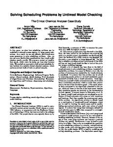
crew schedules. For NS, the software is considered to be a black box where data are inserted and duties are returned. During the years of using the software, we got the impression that although the system was capable of handling quite large instances, the results could be improved using the characteristics of our problem. This was based on two observations. The first observation is that, as explained in the example below, the global constraints are to be validated on a weekly basis. The original method used a static partitioning of the complete problem into separate days of the week. Before a solution was computed an estimate was made on the effect the sub-problem would have on the complete problem. We observed that planning for a complete week and taking into account the real week constraint could lead to a better overall solution. The second observation was that in some cases the solution was improved if, for instance, the solution for one crew base was re-scheduled. For this the duties and tasks for that base were given to the TURNI software and the solution for this smaller problem was better than the original solution. This also indicated that solving the larger instance was becoming difficult for the current implementation. To explain the possible benefits of validating the global constraints on a weekly basis, we present Figure 1. In this figure, a few possible duties are plotted. They are assigned to a certain base (A or B) and have a certain length. The vertical line indicates the moment in the night where no trains are operated. For each individual day all kind of averages are calculated. However, the rules deal with averages over the whole week. E.g. the maximum average duration of the duties for a crew base is 8:00 hours. Originally, based on many years of planner’s experience, this was replaced by a limit of 7:40 hours on the average duty duration of a working day and a limit of 9:30 hours in the weekend. In this way the global average would be approximately 8:00 hours. However, it is obvious that applying these bounds in a rigid way does not guarantee optimality.
Figure 1: Duties example 3
In this paper we will describe how we applied new ways of partitioning, based on the two observations, in order to improve the solution of the CSP. The remainder of this paper is organized as follows. The concept of crew scheduling at NS is explained in more detail in Section 2. We will describe the characteristics of the problem which are used in the iterative approach. In Section 3, we briefly discuss some theory which is the basis for our method. Afterwards, in Section 4, we will present our method and we will analyze some examples of sub-problems that are constructed. The computational results of our method are presented in Section 5. Finally, we finish this paper with some concluding remarks.
2
Crew planning at NS
In Figure 2, we give a schematic overview of the crew planning process for drivers and conductors at NS. Other crew members (at ticketing offices, the call center, mechanics, etc.) fall outside the scope of this paper. The crew scheduling problem (CSP) is the problem of assigning tasks to anonymous duties. These tasks are given by the timetable and by the rolling stock schedule (see Huisman et al. (2005) for a discussion on all planning problems at NS). More formally, a task is the smallest amount of work that has to be assigned to one driver. At NS, a task typically contains one or two trips defined by the timetable. A duty is the work for one crew member from a specific crew base on a certain day. At NS, the crew scheduling process has been split in two stages. First, the crew schedules for the annual plan are constructed. Secondly, the crew rosters are created, where the crew members are assigned to operate the duties. This paper will focus on the first phase, the generation of the duties for the annual plan. This plan deals with a generic Monday, Tuesday and so on. This generic annual plan is modified about 6 times a year as a result of changes in timetable and rolling stock schedules. The other parts of the process fall outside the scope of this paper (for crew rostering, we refer to Hartog et al. (2006) and for crew re-scheduling to Huisman (2007)). In the CSP that is solved for generating the generic annual plan, some rostering aspects are also taken into account. For instance, the average duty length over all duties on a certain crew base should not exceed 8 hours. The reason is that, if this time is exceeded, then it is impossible to construct rosters where the average working time per week is less than 36 hours (in principle each full-time crew member works 9 days in two weeks). The number of night duties (duties with a working period between 1:00h and 5:00h) in a roster is also limited. This constraint should also be validated at a weekly basis. 4
Figure 2: Crew planning process Moreover, it is important that to obtain a fair division of the work over the week for the different crew members, the work should be fairly spread over the different bases. The latter constraints are typical for the Dutch situation and are known as “Sharing Sweet & Sour” rules. They aim at allocating the popular and the unpopular work as fairly as possible among the different crew bases. For instance, some routes are more popular than others and intercity trains are preferred over regional trains. One example is the percentage of work on intercity trains. Of the work assigned to a base for a week, at least 25% should be on the intercity trains. Again, we could require every weekday to contain at least 25% of this work but it is better to check this constraint for a complete week. For a more detailed description of these rules, we refer to Abbink et al. (2005). Finally, notice that the timetables for Monday until Friday are very similar. Therefore, NS uses one (the Friday) of the working days as a pattern working day. At the end, the solution for this working day is used as a solution for the other working days too. The differences between the working days are handled manually. Of course, one should take into account here 5
that for computing the averages over a week the Friday is counted 5 times.
3
Models and Algorithms for CSP
In this section, we give a short overview on models and algorithms that are used to solve the CSP. Moreover, we provide a mathematical formulation for a CSP containing 2 days without tasks overnight. The CSP can be modeled as a set covering problem with additional constraints. If we consider the problem for a whole week where there is only a minor interaction between the different days, we get a special structure of the mathematical program. To show this, we give a mathematical formulation for the problem with two days. Let T 1 and T 2 be the set of tasks for day 1 and 2, respectively. Furthermore, D 1 and D 2 denote the set of duties for these days. The subset Di1 (Di2 ) of D 1 (D 2 ) consists of the set of duties containing task i. The binary decision variables xj (and yj ) indicate whether duty j ∈ D 1 (D 2 ) is included in the solution or not. Every duty j has positive costs cj . Furthermore, let S be the set of additional constraints and let ls and us be the lower and upper bound for constraint s ∈ S. Finally, let vjs (and wjs ) be the weight of duty j ∈ D 1 (D 2 )for constraint s. Then we can formulate this CSP as follows: min
X
cj xj +
j∈D 1
X
(1)
cj y j
j∈D 2
X
xj ≥ 1
∀i ∈ T 1 ,
(2)
yj ≥ 1
∀i ∈ T 2 ,
(3)
∀s ∈ S,
(4)
∀j ∈ D 1 , ∀j ∈ D 2 .
(5) (6)
j∈Di1
X
ls ≤
X j∈D 1
j∈Di2
vjs xj +
X
wjs yj ≤ us
j∈D 2
xj ∈ {0, 1} yj ∈ {0, 1}
Equation (1) is the objective function, which states that the sum of the duty cost is minimized. Constraints (2) and (3) guarantee that for each task i, at least one duty that contains this task is selected. Note that only duties of day 1 (2) can contain tasks of day 1 (2). It may sometimes be better to perform a task more than once. If, for example, the number of tasks going out of a crew base differs from the number of tasks going into the crew base on a 6
day, overcovering is necessary. Moreover, even if overcovering is unnecessary, it may be cheaper to allow overcovering. By allowing overcovered tasks it can be that other tasks can be covered easier, resulting in a larger decrease in costs than the extra money for the overcovered task. Constraints (4) are additional constraints. Consider as an example of an additional constraint, a crew base for which the total number of duties on both days is limited to 50. Then ls = 0, us = 50 and vjs (wjs ) = 1 for all duties belonging to this base and vjs (wjs ) = 0 for all other duties. For some additional constraints it is allowed to violate the constraint at the cost of a penalty. These constraints are moved to the objective function, along with the penalty. The last two sets of constraints (5,6) indicates that the decision variables are binary. Even if the CSPs are solved day by day, the resulting set covering problems are extremely large. TURNI uses column generation combined with a Lagrangian-basic heuristic. This Lagrangian-based heuristic, called CFTheuristic, in which CFT stands for Caprara, Fischetti and Toth, forms the bases of TURNI (see Caprara et al. (1999a)). The main characteristics of the heuristic are a dynamic pricing scheme for the variables, coupled with subgradient optimization and greedy algorithms, and the systematic use of column fixing to obtain improved solutions. To tackle the large number of potential duties, TURNI uses column generation to generate feasible duties (“columns”). These duties are generated by solving a resource constrained shortest path problem in an acyclic network. In this network, the nodes corresponds to the tasks, and there are arcs between two nodes if the two tasks can be assigned to the same crew member. Moreover, a path in the network corresponds now to a feasible duty when it starts and finishes in the same base, and all kind of additional constraints such as duty length and break rules are satisfied. The costs of the arcs are defined such that the total cost of a path is equal to the reduced cost of a duty. By finding the shortest, feasible path and checking whether its cost is negative or not, it is possible to check if there are still duties with negative reduced costs. If not, the column generation is stopped. We refer the reader for details about the theory of column generation to a few recent surveys on this topic: Barnhart et al. (1998); L¨ ubbecke & Desrosiers (2005); Desaulniers et al. (2005). For a more detailed description how TURNI works, we refer to Kroon & Fischetti (2001). The only relevant detail to follow the remainder of the paper, is the fact that the in TURNI output, not only the final set of created duties is presented, but also a large number of “good” duties are available, which are generated throughout the process. We will use this additional information for constructing our sub-cases as described in Section 4.4.
7
4
The partitioning method
As mentioned before, our method is based on two observations. The first observation was that global constraints are to be validated on a weekly basis. The second observation was that in some cases the solution was improved if, for instance, the solution for one crew base was re-scheduled. Combining the two observations, we reasoned that we could possibly improve the overall solution if we would take the solution for one or more bases for the separate days and combine them into a case for the complete week. Furthermore, we reasoned that it would be good to have several iterative combinations of bases in order to reduce the negative effect of optimizing over a sub-problem. We are also interested in the effect of varying the sizes of the cases. The most important dimensions in scheduling are time and location of the activities. It seems natural to use these dimensions to partition the overall problem. We will now describe the four different partitioning methods one by one.
4.1
Weekday partitioning
In this method we create a sub-problem per weekday. All trips belonging to the same weekday are combined in a sub-problem. For the Friday (as representative for a working day), the Saturday and the Sunday a separate solution is created. The advantage of this method is that it can be used without an initial solution. Because tasks of different weekdays cannot be scheduled together in a single duty at NS, this method is a good option to create an initial solution. In fact, this method was used as the only partitioning method during the first years of using the system.
4.2
Geographical partitioning
The primary geographical partitioning is the base to which a duty is created and assigned. After an initial solution is created we can combine all duties assigned to a base for all weekdays. This results in 29 sub-problems, one for each base. These sub-problems are very small and do not provide much room for improvement. Therefore, we create some larger cases by clustering some bases based on the geographical location. For this, we split the country into a number of equally sized regions. We create small partitions where on average 3 bases are clustered and we create large partitions where on average 7 bases are clustered.
8
4.3
Line based partitioning
The railway product is defined by railway lines. Trains are operated along several railway lines at a certain frequency. For example, consider the 800 line in Figure 3. This line passes through several bases, which can be grouped into one cluster. We have done this for 4 important long-distance lines, obtaining four clusters.
Alkmaar Amsterdam Utrecht Den Bosch Eindhoven
Heerlen Maastricht
Figure 3: The 800-line with adjacent bases
4.4
Partitioning based on column information
The last partitioning method we present is based on the information that is generated by the scheduling algorithm. As indicated in Section 3, TURNI uses a mechanism to rank duties according to their likelihood to be selected in an optimal solution. In this way good duties are created which have a high probability to be part of the optimal solution. Duties that have no contribution to a good solution are removed from the set, while new duties that have a positive contribution are added. Therefore the total set of duties is continually improving. TURNI not only returns the duties which are in the final solution, but it also returns these good duties which were generated 9
during the solution process. These duties can be used to give the information we look for. If two tasks appear together in many duties, it is likely that these two tasks will be assigned to the same duty in the optimal solution. If, on the other hand, two tasks (almost) never appear together in a duty, these tasks will probably be assigned to different duties in the optimal solution. Now, it is possible to give each pair of duties in the current solution a score which can be used as a measure for inserting a pair into a partition. This score is based on how often tasks from these two duties appear together in the set of all duties. We calculate the score for each pair as follows. First, we count for each combination of tasks in these duties, say t1 and t2 , the number of duties in the whole set that covers task t1 and t2 . Then, we add all these numbers. In this way, we can construct a graph G = (V, E), where the duties are represented by the vertices, and the edges represent the fact that the score is positive. We define a weight q(u, v) for each edge (u, v) ∈ E. This weight corresponds to the score calculated above. We want to find a partition of the vertices of G into k equal subsets V1 , ..., Vk , such that the total weight of the edges between different subsets is minimized, or more formally X min q(u, v). (7) (u,v)∈E,u∈Vi ,v∈Vj ,i6=j
We use a generic algorithm for graph partitioning based on Kernighan & Lin (1970) to solve this problem. For the details, we refer to Van ’t Wout (2007).
5 5.1
Results Experimental Design
All experiments were carried out on the same hardware (Intel Quoad Core, 2.6GHz, 4Mb RAM). First we evaluated the different partitioning methods by running them after a base run in which we used the weekday partitioning. We set up several experiments in which we tested the performance of a partitioning method based on the results of the base run. Next to that we have performed experiments in which all methods were applied sequentially. We terminated TURNI with solving a sub-problem if there was no improvement anymore. The results we obtain are based on both optimizing over the week constraints and on iteratively solving smaller sub-problems. To evaluate both aspects, we also performed runs in which we did not optimize over the week but only applied the method on separate weekday cases. Furthermore, we 10
wanted to evaluate the method for both drivers and conductors, so we made separate experiments for them.
5.2
Computational results
In the Tables 1-4, we present the results of the experiments. The first line corresponds to the different partitioning methods explained in Section 4 that we applied: • weekday partitioning (columns “Day”), • geographical partitioning with about 7 bases together (columns “Geo L”), • geographical partitioning with about 3 bases together (columns “Geo S”), • line based partitioning (column “Line”) • partitioning based on column information (columns “Info”). The numbers in the columns corresponding to the different methods indicate the order in which the methods are applyied. An empty cell indicates that the method was not used in the experiment. In the last two columns, we report the number of duties and the relative improvement compared to the base case. We choose to report the number of duties instead of the objective function, because the value of the objective function is mainly determined by the number of duties. The first series of experiments, as reported in Table 1, deal with a driver’s instance (all trips to be operated by the drivers for a complete week) and a limit on the average duration of 7:40h for the weekday and 9:30h for the Saturday and Sunday. In these experiments, we have not relaxed any of the global constraints meaning that we have dealt with the real-world problem. Moreover, in these experiments, we applied only the partitioning to the individual days. In other words, we have not optimized over the week constraints. We can see that the partitioning method shows a significant reduction in the number of duties (1.8%). Applying the sequence of partitioning methods does not improve the solution compared with only the geographic partitioning. The second type of experiments (Table 2) also deal with the same driver’s instance as in the previous experiments. The differences are that the constraints on variation and number of duties are relaxed, and that we optimized over the whole week. We can see in these experiments that the initial solution is worse although several constraints are relaxed. It seems that this is 11
1 2 6
Day Geo L 1 1 2 1 2
Geo S
Line
Info
3
4
5
#Duties Av. Dur. 6072 7:31 5964 7:37 5964 7:45
∆Duties -1.8% -1.8%
Table 1: Results of a week instance for drivers with all constraints difficult for the TURNI algorithm. Therefore, the potential improvement is larger, which is also achieved by the partitioning methods. The final solution is even better than in the first range of experiments, which could also be expected because some constraints are relaxed. 1 2 6
Day Geo L 1 1 2 1 2
Geo S
Line
Info
3
4
5
#Duties Av. Dur. 6180 7:39 5969 7:54 5944 7:54
∆Duties -3.4% -3.8%
Table 2: Results of a week instance for drivers based on different average durations The third range of experiments shown in Table 3 is again the instance for drivers. These experiments were similar to the previous ones except that we have used a maximum average duration of 8:00h for all sub-problems. Compared to the previous range of experiments, we can see that the initial solution is worse because the wrong maximum average duration is chosen. We can see that the partitioning method works very well giving an overall efficiency improvement of 4.2% after sequentially applying all methods. We can also see that the second partitioning method has the largest efficiency improvement if you apply it after the weekday instances. Unfortunately, although the relative improvement is larger, we do not get such a good solution as in the previous experiments. It seems that the bad solution of the weekday runs has its effect on the final solution. This indicates that making a good guess on the average in the weekday instances has a significant effect. This guess was based on the experience of the planners who seem to be right. The last set of experiments, presented in Table 4, is on an instance for conductors (all trips to be operated by the conductors for a complete week). This instance has 18,000 trips compared to 15,000 for the drivers, because on several trains two conductors are required. In these experiments we used the averages 7:40h for the weekday and 9:30 for the Saturday and Sunday as used in the planning of the previous years. Next to that we have applied the very tight constraints on the number of duties per base. In this case we did apply the optimization over the week constraints. We can see that two 12
1 2 3 4 5 6
Day Geo L 1 1 2 1 1 1 1 2
Geo S
Line
Info
2 2 3
4
2 5
#Duties Av. Dur. 6235 7:43 6006 7:53 6045 7:54 6022 7:53 6064 7:50 5971 7:54
∆Duties -3.7% -3.0% -3.4% -2.7% -4.2%
Table 3: Results of a week instance for drivers based on an average duration of 8:00h a day methods outperform the solution were we apply all methods sequentially. The best results are obtained by applying the partitioning into small geographical oriented sub-problems. It seems that due to the fact that the conductors case is larger than the drivers case, it helps to reduce the size of the sub-problems by using the small geographical partitioning which creates the smallest subproblems compared to the other methods. 1 2 3 4 5 6
Day Geo L 1 1 2 1 1 1 1 2
Geo S
Line
Info
2 2 3
4
2 5
#Duties Av. Dur. 7432 7:49 7339 7:56 7318 7:55 7335 7:56 7331 7:54 7335 7:57
∆Duties -1.3% -1.5% -1.3% -1.4% -1.3%
Table 4: Results of a week instance for conductors with all constraints Overall we see that we all partitioning methods give more or less the same results. By applying them all after each other, the largest improvement can be gained. Moreover, this approach has as advantage that parallel computing can be applied such that the throughput time of the whole process can be reduced. This can speed up the whole crew scheduling process to a large extend. The best solution of the iterative partitioning methods was implemented in practice for the crew schedules corresponding to the timetable of the year 2007. Together with some other small improvements in the process, this has led to an efficiency improvement of about 2%. In this way, the expected shortage of crew was solved and a total saving of about 6 million euro was achieved.
13
6
Conclusions
In this paper, we described a method that improved the usage of an advanced crew scheduling algorithm using iterative partitioning of the problem. The method is being used to create a weekly crew schedule for drivers and conductors. We have shown that applying some basic partitioning techniques can have a significant added value when combined with an advanced crew scheduling algorithm. Overall the efficiency was improved with almost 2%. In this way, the expected shortage for the 2007 timetable could be reduced significantly such that the timetable went smooth in operation. The method is automated which not only enables us to create an efficient production plan, but also gives us the possibility to use it for what-if scenario analysis. In the past the scenarios were only studied for a single weekday. With this method, the analysis are more reliable because the complete week is taken into account.
References Abbink, E., Fischetti, M., Kroon, L., Timmer, G., & Vromans, M. 2005. Reinventing crew scheduling at Netherlands Railways. Interfaces, 35, 393– 401. Barnhart, C., Johnson, E.L., Nemhauser, G.L., Savelsbergh, M.W.P., & Vance, P.H. 1998. Branch-and-Price: Column Generation for Solving Huge Integer Programs. Operations Research, 46, 316–329. Caprara, A., Fischetti, M., & Toth, P. 1999a. A Heuristic Algorithm for the Set Covering Problem. Operations Research, 47, 730–743. Caprara, A., Fischetti, M., Guida, P.L., Toth, P., & Vigo, D. 1999b. Solution of Large-Scale Railway Crew Planning Problems: the Italian Experience. Pages 1–18 of: Wilson, N.H.M. (ed), Computer-Aided Transit Scheduling. Springer Verlag, Berlin. Desaulniers, G., Desrosiers, J., & Solomon, M.M. (eds). 2005. Column Generation. Springer, New York. Desrosiers, J., Dumas, Y., Solomon, M.M., & Soumis, F. 1995. Time Constrained Routing and Scheduling. Pages 35–139 of: Ball, M.O., Magnanti, T.L., Monma, C.L., & Nemhauser, G.L. (eds), Network Routing. Handbooks in Operations Research and Management Science, vol. 8. NorthHolland. 14
Fores, S., Proll, L., & Wren, A. 2001. Experiences with a Flexible Driver Scheduler. Pages 137–152 of: Voß, S., & Daduna, J.R. (eds), ComputerAided Scheduling of Public Transport. Springer, Berlin. Hartog, A., Huisman, D., Abbink, E.J.W., & Kroon, L.G. 2006. Decision Support for Crew Rostering at NS. Tech. rept. EI2006-04. Econometric Institute. Hoffman, K.L., & Padberg, M. 1993. Solving Airline Crew Scheduling Problems by Branch-and-Cut. Management Science, 39, 657–682. Huisman, D. 2007. A Column Generation Approach to solve the Crew ReScheduling Problem. European Journal of Operational Research, 180, 163– 173. Huisman, D., Kroon, L.G., Lentink, R.M., & Vromans, M.J.C.M. 2005. Operations Research in passenger railway transportation. Statistica Neerlandica, 59, 467–497. Kernighan, B., & Lin, S. 1970. An Efficient Heuristic Procedure for Partitioning Graphs. Bell Systems Technical Journal, 29, 291–307. Kohl, N. 2003. Solving the World’s Largest Crew Scheduling Problem. ORbit, 8–12. Kroon, L.G., & Fischetti, M. 2001. Crew Scheduling for Netherlands Railways ”Destination: Customer”. Pages 181–201 of: Voß, S., & Daduna, J.R. (eds), Computer-Aided Scheduling of Public Transport. Springer, Berlin. L¨ ubbecke, M.E., & Desrosiers, J. 2005. Selected Topics in Column Generation. Operations Research, 53, 1007–1023. Van ’t Wout, J. 2007. Crew Scheduling at Netherlands Railways: using TURNI effectively. M.Sc. thesis, Faculty of Economics, Erasmus University Rotterdam.
15