SOLVING MULTI-OBJECTIVE MODELS WITH GAMS

SOLVING MULTI-OBJECTIVE MODELS WITH GAMS ERWIN KALVELAGEN

Abstract. Some classes of Multi-objective models can be implemented as either a single linear programming model or a series of linear programming models. This document shows how this can be done in a GAMS environment.

1. Multi-objective programming GAMS models have a single objective. In some cases a problem may require a so-called multi-objective formulation: different objectives need to be optimized. Mathematically a multi-objective programming problem can be stated as:  z1 = cT1 x      z2 = cT2 x MOLP minimize .. x   .    zK = cTK x subject to Ax ∼ b `≤x≤u

where ∼ is a vector of relational operators {≤, = . ≥}. In the above model we have K objectives. This model can not be cast directly as a linear programming problem without making some assumptions. The easiest way to deal with this problem is to create a linear weighted objective: (1)

min z 0 =

K X

wi zi

i=1

The problem here is to find a suitable set of weights wi . Specifying weights is especially difficult if the objectives have different units (i.e. combining a profit criterion with a customer satisfaction quantity). This linear weighted objective is an example of a value or utility function (2)

min z 0 = Ψ(z)

Such functions are sometimes called ’scalarizing functions’ [9]. As an example we mention the portfolio optimization problem where both return and risk need to be optimized. For these problems often a linear combination of the two objectives is used. A multiple objective capital budgeting model based on this technique is described in section 4. For an example of a multiple objective model in water allocation modeled along these lines in GAMS see [10]. If the K objectives follow a dominance order, i.e. objective k should be optimized first, before considering the value of objective j, then we can implement a simple Date: September 20, 2002. 1

2

ERWIN KALVELAGEN

sequential algorithm. This particular model is called lexicographic. We assume that the objectives are ordered such that zi dominates zj when i < j. We can now formulate the algorithm: for j := 1 to K do solve min zj , zi = cTi x, Ax ∼ b, ` ≤ x ≤ u add constraint zj = zj∗ to the problem end for In GAMS such an algorithm can be expressed quite easily: alias (i,j); parameter p(i) ’selection of objective’; equation objective ’select correct z by assigning to p’; objective.. obj =e= sum(i,p(i)*z(i)); model m /all/; loop(j, * select correct objective function p(i) = 0; p(j) = 1; * solve problem solve m using lp minimizing obj; * add fixed objective z.fx(j) = z.l(j); );

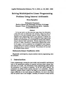
A variant is to allow the higher priority objectives to deviate ε% from their optimal value. In this case the method is called a hierarchical optimization method. The techniques describes in this section extend directly to mixed integer and nonlinear programming models. The general MOLP problem, where there is no dominance and no utility function Ψ(.) is available, is not directly solveable as an LP. The problem is that there are an enormous number of efficient or Pareto-optimal solutions of which the modeler needs to choose from. Pareto-optimal solutions are solutions that can not be improved with respect to an objective zi without deteriorating another objective zj . Specialized MOLP solvers often use an interactive approach, that requires interaction of the modeler during the solution process. They ask questions to the modeler in order to guide him or her through the set of efficient solutions such that a preferred solution can be found. Recently there has been significant interest in using genetic programming for problems with multiple objectives [2]. In general these solvers are aimed for small problems. GAMS and the solvers supported by GAMS does not have facilities for these solution procedures. More information can be found in for instance [13], [1]. 2. Goal programming A special form of multiple objective programming is goal programming[4]. Goal programming deals with multiple, possibly conflicting goals, which may be measured in nonhomogeneous units. An objective fi (x) is reformulated into a goal by considering an aspiration level bi . Goals can have the form fi (x) ≤ bi , fi (x) = bi or − fi (x) ≥ bi . After adding slacks or deviations s+ i ≥ 0 and si ≥ 0, we can minimize appropriate slacks to try to achieve the goals. The formulation of these slacks is summarized in table 1.

SOLVING MULTI-OBJECTIVE MODELS WITH GAMS

3

Goal Type Goal Programming Form Slacks to be minimized − fi (x) ≤ bi fi (x) − (s+ s+ i − si ) = bi i + − fi (x) ≥ bi fi (x) − (si − si ) = bi s− i − − fi (x) = bi fi (x) − (s+ s+ i − si ) = bi i + si Table 1. Goal programming formulations

The term non-preemptive goal programming is used when we can model the problem by using linear weights on the deviations to construct a single objective. Preemptive goal programming assumes a strict dominance order of the goals, which can be solved using a sequence of linear programming problems as described in the previous section. In the context of goal programming this algorithm is called Sequential Linear Goal Programming (SGLP) (somehow the order is mixed up in the acronym). An example of a preemptive goal programming formulation of a budget allocation problem is described in section 6. For more information on goal programming see the following references: [3], [4], [11], [12]. 3. The Capital Budgeting problem The Capital Budgeting problem is related to the knapsack problem [14]. The goal is to select projects to invest in, such that benefits are maximized. A project i will need a capital expenditure Ci . The benefits of investing in project i are realized over the lifetime of the project, and are denoted by bi,t . We can use a standard net present value calculation to find the current value of these cash flows: X bi,t (3) Bi = (1 + r)t t where r is the interest rate. These calculations are carried out on constants, and are not part of the decision model itself. The model therefore does not become nonlinear because of the net present value calculations. Assuming a total budget of C we can write the model as: X CAP BUDGET maximize Bi xi x i X subject to Ci xi ≤ C i

xi ∈ {0, 1} ∀i where xi is a binary variable indicating whether project i is selected. If there are projects that are mutually exclusive, then we can add constraints of the form: X (4) xi ≤ 1 i∈S

where S is the set of mutually exclusive projects. If a project k is contingent on selection of project j, we can add: (5)

xk ≥ xj

4

ERWIN KALVELAGEN

Financial Present Value Resource Efficiency Quality Facility Quality

Present value of incremental cash flows. Enhances employee productivity.

Improves facility’s appearance or usefulness, including expenditures to meet safety, code, or accreditation standards. Patient/Family Satisfaction Improves patients’ clinical experience by lowering waiting times, throughput times. and general comfort. Patient Outcomes Improves patients’ clinical outcomes. Physician Relationships Increases physicians’ satisfaction by improving equipment reliability, introducing newer technology, and/or enhancing physicians’ efficiency of effectiveness. Strategic Information Integration Promotes integration of data/information within the hospital or healthcare system, between hospital and physician, and with other healthcare entities. Market Share Enhances market share by increasing patient volume and/or attracting new patients. Table 2. Attributes for project proposals

A constraint like (6)

xk = xj

would implement a mutual contingency: either both projects j and k are selected or neither of them. 4. A multiple objective capital budgeting model The following model is a capital budgeting problem that has multiple objectives [8]. The model is concerned with allocating budget to project proposals in a hospital setting. Projects are not only evaluated according to their Present Value (PV) but also other attributes play a role. For each project proposal scores are given for each of the attributes presented in table 2. The table is taken from [8]. Some of the attributes can be measured such as Present Value, but others are more subjective and need to be determined by the modeler and subject matter specialists. This model uses a scalarizing function with linear weights (see section 1). The weights need to be determined by the modeler, again in most cases with help by subject matter specialists. In the model a few interesting issues arise. First we have instances of nondiscretionary spending. Some projects need to be selected because they addressed safety concerns, regulatory standards, or prior contractual agreements. Secondly, there are projects that are mutually exclusive (equipment upgrades by competing vendors) or mutually contingent.


5

Notice that the data entry for mutually contingent projects is simplified by creating a set MC. However this is not convenient for writing the constraints of the form xi = xk . Therefore we create two sets MCLHS and MCRHS which make the specification of the equations trivial. This illustrates the modeling paradigm of making equations as simple as possible. An important additional advantage is that we can debug the sets MCLHS and MCRHS by displaying them. We don’t need a complete model before we can do this. The equation MUTCONT is now so simple we can basically assume it is correct once we have made sure the sets MCLHS and MCRHS are correct. If this was not the case we would need to look at the equation and column listing in the listing file, which is only available after we can generate a complete model. It is noted that mutually contingent projects need to be specified pairwise. I.e. if there are three mutually contingent projects xi , xj and xk , then we need to specify this in two pairs, e.g. (xi , xj ) and (xi , xk ). The model shows a significant amount of data manipulation: a small part of the GAMS source is devoted to specifying the model equations perse. This is not unusual for practical models. 4.0.1. Model capbudget.gms. $ontext A multi-objective capital budgeting model for a hospital Erwin Kalvelagen, July 2002 Reference: Don N. Kleinmuntz, Catherine E. Kleinmuntz, "Multiobjective capital budgeting in not-for-profit hospitals and healthcare systems", tech report, december 2001. $offtext set i ’projects’ / p1 ’Ultrasound Siemens Upgrade’ p2 ’INTRAOPERATIVE MONITORING EQUIPMENT’ p3 ’Central Data Repository’ p4 ’Communication Closets/Cabling’ p5 ’Radiology Digital Fluoro’ p6 ’Clinical Information system’ p7 ’Centralized Scheduling’ p8 ’Upgrade Pneumatic Tube System - All Bldgs’ p9 ’Mobile/Radio frequency computers’ p10 ’Ultrasound Acuson Upgrade’ p11 ’Pneumatic Tube, Point to Point’ p12 ’Remodeling of Immediate Care Center’ p13 ’Birthing Center Expansion’ p14 ’Medical Vacuum Pumps - CCB’ p15 ’Adult Ventilators’ p16 ’Cardiac Cath Lab Renovation and Upgrade’ p17 ’Radiology Portable C-Arm’ p18 ’MRI Patient Monitors’ p19 ’ACB Pharmacy Renovation’ p20 ’SMS Product Line Manager’ p21 ’SMS Imaging’ p22 ’Echocardiograph’ p23 ’OP Rad/fluoro rooms’ p24 ’Replace Oxyquip Medical Gases outlets - CCB’ p25 ’Doors for all OR rooms’ p26 ’Human Resource/Payroll Information System’ p27 ’Anesthesia Machine Modulus SmartVent System’ p28 ’ABIOMED EXTERNAL ARTIFICAL HEART PROGRAM’ p29 ’Replace all 486 computers’ p30 ’Robot-Rx’ p31 ’EXTERIOR SIGNAGE’

6

p32 p33 p34 p35 p36 p37 p38 p39 p40 p41 p42 p43 p44 p45 p46 p47 p48 /;

ERWIN KALVELAGEN

’Powervision 6000 Digital Ultrasound System’ ’Z-Kat Fluorotactic Guidance System’ ’Audiovisual Upgrades - 831’ ’ORSOS Upgrade’ ’PLC LASER’ ’Replace Kathabar Air Handling Units 13 & 14 - CCB’ ’PACs Radiology’ ’IV Room Remodeling Pharmacy’ ’AS/3 Anesthesia Monitors’ ’Refurb CPS 8th Floor CCB’ ’Unified Messaging’ ’Push Messaging System’ ’Patio Cafe Construction and Refurb’ ’Beds’ ’7th,8th,9th Floor (East & South Wings Units) Renovation’ ’Add Sprinkler System - ACB - Second Phase’ ’Ambulatory Surgery Center’

set attr ’attributes’ / * financial attributes PV ’present value of incremental cash flows’ EFF ’resource efficiency: employee productivity’ * quality attributes FQ ’facility quality: appearance or usefulness, incl. safety, code, accreditation standards’ SAT ’patient and family satisfaction’ OUTC ’patient clinical outcome’ PHYS ’physician satisfaction’ * strategic IINT ’Information Integration’ SHAR ’Market share’ /;

table score(i,attr) ’attribute scores’ PV EFF FQ SAT OUTC p1 0 2 0 1 3 p2 0 2 0 2 4 p3 0 2 0 1 0 p4 0 9 1 0 6 p5 0 1 0 0 0 p6 0 26 1 3 14 p7 0 9 1 2 2 p8 0 4 0 2 4 p9 0 2 0 1 2 p10 0 0 0 0 0 p11 0 3 1 1 4 p12 2232525 14 12 7 9 p13 5079297 100 100 100 100 p14 0 7 2 1 10 p15 0 0 0 0 0 p16 2153191 54 13 16 41 p17 0 4 1 1 5 p18 0 0 0 0 0 p19 998542 14 6 7 0 p20 0 78 0 4 0 p21 554746 14 0 2 5 p22 0 9 2 2 10 p23 1502436 14 3 9 25 p24 0 4 2 1 4 p25 0 2 0 0 1 p26 0 8 0 0 2 p27 0 13 5 2 29 p28 164428 18 10 7 24 p29 -638885 5 0 0 2 p30 210341 59 19 17 0 p31 0 0 0 0 0 p32 0 0 0 0 0 p33 0 0 0 0 1

PHYS 3 5 5 9 2 21 7 2 3 0 1 7 100 7 0 0 4 0 11 62 0 7 0 4 2 0 29 0 1 0 0 0 1

IINT 0 2 7 19 0 50 11 3 2 0 2 0 0 0 0 75 0 0 0 100 70 0 15 0 0 8 13 0 8 55 0 0 0

SHAR 2 2 1 3 1 8 5 2 1 0 1 11 100 1 0 8 2 0 8 8 7 6 9 0 1 0 8 22 0 25 0 0 1


p34 p35 p36 p37 p38 p39 p40 p41 p42 p43 p44 p45

0 0 831553 0 832118 0 0 0 0 0 0 0

0 0 8 0 31 0 0 0 0 0 0 0

0 0 0 0 0 0 0 0 0 0 0 0

0 0 4 0 8 0 0 0 0 0 0 0

0 0 20 0 21 0 0 0 0 0 0 0

0 0 0 0 0 0 1 0 0 0 0 0

1 0 0 0 50 0 0 0 0 0 0 0

0 0 8 0 0 0 0 0 0 0 0 0

; * * some projects are non-discretionary * set nd(i) ’non-discretionary projects’ /p46,p47,p48/; set d(i) ’discretionary projects’; d(i) = not nd(i);

* * we scale the scores from 0 - 100 * parameter minscore(attr) ’minimum score’; minscore(attr) = smin(d, score(d,attr)); parameter maxscore(attr) ’maximum score’; maxscore(attr) = smax(d, score(d,attr)); parameter scaled_score(i,attr); scaled_score(d, attr) = 100*(score(d,attr)-minscore(attr))/(maxscore(attr)-minscore(attr)); display scaled_score; * * the weights for the different attributes * parameter weight(attr) / PV 100 EFF 100 FQ 50 SAT 75 OUTC 70 PHYS 45 IINT 50 SHAR 100 /;

scalar sumw ’sum of weights’; sumw = sum(attr, weight(attr)); parameter w(attr) ’normalized weights’; w(attr) = weight(attr)/sumw; display w;

* * calculate weighted value scores * (these results are slightly different than in the * reference) * parameter val(i) ’weighted value scores’; val(i) = sum(attr, w(attr)*scaled_score(i,attr)); display val;

parameter cost(i) ’cost of each project’ / p1 76896, p2 120000, p3 112000, p4 p6 500000, p7 225000, p8 154280, p9

225000, p5 125000, p10

80049 76896

7

8

p11 144241, p12 p16 1500000, p17 p21 700000, p22 p26 250000, p27 p31 128004, p32 p36 734464, p37 p41 190803, p42 p46 2620000, p47 /;

ERWIN KALVELAGEN

683382, 192576, 362000, 803975, 128004, 150000, 250750, 300000,

p13 3935679, p14 p18 90960, p19 p23 914000, p24 p28 863509, p29 p33 150000, p34 p38 1500000, p39 p43 420500, p44 p48 5125000

235244, 525000, 210900, 122756, 145910, 171500, 450050,

p15 90000 p20 1500000 p25 150000 p30 1643576 p35 140000 p40 209125 p45 779925

* * the available budget limits the number of projects that can be * carried out. * parameter budget ’in millions’ / 15.8 /; * * mutually exclusive projects * In this case projects 1 and 10 are equipment upgrades from * competitive vendors. * set mes ’number of mutually exlusive sets’ /me1/; set me(mes,i) ’specification of mutually exclusive projects’ / me1.(p1,p10) /; * * mutually contingent projects * need to be specified in pairs * set mcs ’number of mutually contingent sets’ /mc1/; set mc(mcs,i) ’specification of mutually contingent projects’ / mc1.(p20,p21) /;

loop(mcs, abort$(sum(mc(mcs,i),1)2) "The set mc need to be specified in pairs"; ); * * create a set mclhs and mcrhs for easier writing of the equations * set mclhs(mcs,i); mclhs(mc) = no; set mcrhs(mcs,i); scalar lhs; loop(mcs, lhs = 1; loop(mc(mcs,i), if (lhs, mclhs(mc) = yes; lhs = 0; else mcrhs(mc) = yes; ); ); ); display mclhs, mcrhs; variables z ’objective’ x(i) ’project selection’ ; binary variable x; equations objective ’objective function’ budgetcon ’budget constraint’ mutexcl(mes) ’mutually exclusive projects’ mutcont(mcs) ’mutually contingent projects’ ;


9

* * non-discretionary projects need to be selected * x.fx(nd) = 1; * * objective: maximize value * objective.. z =e= sum(i, val(i)*x(i)); * * budget constraint * budgetcon.. sum(i, cost(i)*x(i)) =l= budget*1.0e6; * * mutually exclusive projects: only one can be selected from * sets. * mutexcl(mes).. sum(me(mes,i), x(i)) =l= 1; * * mutually contingent projects: all projects in sets need to * selected together * mutcont(mcs).. sum(mclhs(mcs,i), x(i)) =e= sum(mcrhs(mcs,i), x(i)); model m /all/; option optcr=0; solve m maximizing z using mip; option x:0; display x.l;

The solution of this model is as follows: ---p1 p9

1, 1,

295 VARIABLE x.L p2 1, p12 1,

p3 1, p13 1,

project selection p4 1, p16 1,

p5 1, p46 1,

p6 1, p47 1,

p7 1, p48 1

p8

1

For a related model see [6].

5. A multiple objective assignment problem The problem we describe here is based on a client model1. Many countries have sizeable governmental statistical offices. Although there is a trend to downsize them, by using information technology, data communication, better use of available registers such as tax records, and smarter sampling techniques, old fashioned faceto-face interviews are still considered a valuable way to collect data. In this study we want to assign interviewers to respondents. We assume there is a large collection of respondents and we have choose among them. Interviewers can only travel a certain distance per trip, and can carry out a limited number of interviews. The objective is to maximize the number of respondents to be interviewed while minimizing the total distance traveled.

1The model was proposed by Maarten Schuerhoff

10

ERWIN KALVELAGEN

The basic model looks like: min td =

X

di,j xi,j

i,j

max nr =

X

yj

j

yj =

X

(7)

xi,j

i

X

xi,j ≤ maxi

j

xi,j = 0 for di,j > maxd xi,j ∈ {0, 1} yj ∈ {0, 1} As the total possible number of respondents is very large the number of variables xi,j becomes very large. We can make the model manageable by dropping from the model all variables xi,j with di,j > maxd. In the solution procedure we first solve to maximize the number of respondents that can be reached, and subsequently we minimize the total distance. Notice that changing the order is not an option. If we would first minimize the total distance, we would end up with no interviews being done. Both models can be solved as LP’s as the solution is automatically integer, which is very helpful in keeping the solution time down. 5.0.2. Model interview.gms. set i ’interviewers’ / 20007 20027 20031 21021 21106 21109 21116 49001 95012 96010 98002 98038 99012 /; set j ’respondents’ / $offlisting $include respset.csv $onlisting /;

parameter dist(i,j) ’distances’ / $offlisting $ondelim $include dist2.csv $offdelim $onlisting /; scalar maxassign ’max number of respondents for each interviewer’ /25/; set ij(i,j) ’subset of allowed assignments’;


set jj(j) variables x(i,j) tdist y(j) nr ;

’eligible respondents’;

’assignment enqueteurs -> respondents’ ’total distance’ ’active respondents’ ’numer of respondents’

binary variables x,y; parameter maxdist(i); equations totdist calcy(j) mxassign(i) numresp numrespfx ;

’total travel distance’ ’calc number of active respondents’ ’max 25 respondents for each interviewer’ ’number of respondents (objective)’ ’number of respondents (fixed)’

totdist.. numresp.. numrespfx.. calcy(jj).. mxassign(i)..

tdist =e= sum(ij, dist(ij)*x(ij)); nr =e= sum(jj, y(jj)); nr.l =e= sum(jj, y(jj)); y(jj) =e= sum(ij(i,jj), x(ij)); sum(ij(i,j), x(ij)) =l= maxassign;

model m1 /numresp,calcy,mxassign/; model m2 /totdist,numrespfx,calcy,mxassign/;

set iter /iter1*iter4/; parameter maxdistance(iter) / iter1 5, iter2 10, iter3 20, iter4 50 /;

option rmip = cplex; option limrow=0; option limcol=0; option reslim=10000; option iterlim=1000000; m1.solprint = 0; m2.solprint = 0;

loop(iter, x.l(i,j) = 0; y.l(j) = 0; ij(i,j) = no; ij(i,j)$(dist(i,j)